2.2. Molecular Models

Simulation results are only as good as the potentials (forces) that are used. It is not an easy problem to get accurate forces because the origin of forces is quantum mechanics, to date a computationally intractable problem, but there has been some recent progress. The most common approach is semi-emprical: a functional form is guessed and parameters in the form are deduced from theory or fitted from data. How do we define the potential to be used in MD?

2.2.1. Where Do You Get Potentials?

From First Principles: The Born-Oppenheimer Potential

The fundamental description is in terms of the non-relativistic Schroedinger equation for both the ionic and electronic degrees of freedom. But since the electrons are much lighter they respond more-or-less instantly to the ionic motion. Also typical temperatures are very cold compared to the electronic energy scale (1 Hartree, which sets the scale of the electronic energy, equals 316,000 K) so the electrons are in or close to their ground state. In the Born-Oppenheimer (BO) approximation we fix the ions (and neglect the nuclear kinetic energy) and solve (or try to solve) for the electronic ground state energy. Corrections to BO are usually very small because corrections go as the ratio of the electron to nuclear mass which is smaller than 0.0001 for all atoms except hydrogen and helium. Unfortunately solving for the quantum mechanics is not very easy to do. We will describe some attempts when we discuss quantum Monte Carlo. The other methods are the local density functional theory (and improvements such as the GGA theory), quantum chemistry methods such as Hartree-Fock theory and the configuration interaction method.

One break-though occurred in the late 1980’s when Car and Parrinello (CP) showed how one could simultaneously solve the LDA equation for the electronic energy and the dynamical equations for the nuclei (see, Phys. Rev. Lett. 55, 2471 (1985)). This means one does not have to tabulate the BO energy but just compute it as the ions move. We will describe this method later in the course but the CP approach is very much slower than using fitted potentials (about 4 orders of magnitude). The largest CP studies have several hundreds of electrons or atoms while the largest MD simulation have millions of particles.

Unless we use the CP approach then we have to assume some form for the potential. The assumption of a potential is a big approximation because the potential energy surface is a function of 3N variables for N ions. Symmetries such as translational degrees or rotational of freedom will only get rid of a few degrees of freedom. What usually has to be done is to assume the many-body potential is a sum of pair potentials and perhaps three-body potentials etc. This also assumes the molecule is rigid and weakly interacting with the environment so its internal electronic and vibronic state does not couple with surrounding molecules. A pair potential is a function of a single variable; there is no way it can exactly represent a 3N dimensional function.

Luckily for computer simulation, basic intermolecular structure depends overwhelmingly on two features of the interaction: the shape of the molecules and their long-range interactions due to Coulomb forces. These are not difficult to determine from experiment.

So where do we get the pair potentials from? The basic input is theoretical as we will discuss. The other input is empirical. Some sources of experimental data are:

• atom-atom scattering in the gas phase can give direct information about the atom-atom potential. The scattering energy samples different regions of the interaction depending on the energy of the colliding atoms. gas phase data, for example the virial coefficients and transport properties give integrals over the potential. the low temperature thermodynamic properties. Most materials (except helium) form a solid at low temperature. If the energy as a function of density is known, that gives fairly direct information about the depth of the potential well and its curvature.

• High pressure information. This samples the interaction at shorter distances than at lower pressures. thermodynamic data, such as melting temperature, the critical point and the triple point. This information is harder to use directly as it is many-body property. But one can use simulations to compute a phase diagram with a trial potential, then try to change the potential using perturbation theory to make the trial phase diagram agree with the actual phase diagram.

• One should keep in mind the difference between interpolation and extrapolation. If experimental information is used to determine the potential, it will be good in a nearby region of phase space and for similar properties. But that potential could be quite bad for unrelated properties or outside the region that has been fitted. For example, if the potential has been determined using bulk properties, there is no reason to think it will be good to compute surface properties because the local environment on a surface is not as symmetrical as in the bulk.

Example: Atoms in a Solid

Suppose we consider a “bonding” type atomic interaction in a solid phase. What properties must the analytic form of the potential function be required minimally to mimic some “real” behavior? A small list of properties that we might wish to represent, for example, could be:

• Lattice constant, \(a_0\) (Position of the minimum in the potential.)

• Bulk Moduls, \(K\) (Curvature of potential at \(a_0\).)

• Coefficient of thermal expansion, \(E\) (Asymmetry of potential gives temperature dependence of \(a_0\).)

• Cohesive energy, \(E_c\).

Then, for example, does the simulation reproduce the melting temperature, \(T_m\)?

2.2.2. Two Complementary Approaches to Designing Models

• Use experimental data, invent a model to mimic the problem (semi-empirical approach). But: one cannot reliably extrapolate the model away from the empirical data.

• Use foundation of physics (Maxwell, Boltzmann, and Schrödinger) and numerically solve the mathematical problem, determine the properties (first-principles/ab initio methods)

2.2.3. Classical Atomistic Models

• One Atom is treated as 1 particle

• Interactions with in a molecule, i.e, Intramolecular forces are bonded interactions, angles and dihedrals (or torsional angles) as illustrated in Fig. 2.1.

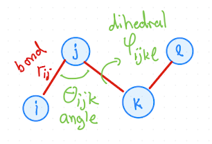
Fig. 2.1 Visualization of bonds, angles, and dihedrals in a molecule with four atoms.

2.2.3.1. Bonded interactions

For example a harmonic bonds can be used. Also see intramolecular potentials.

2.2.3.2. Non-bonded interactions

Energy (\(E= T+V\)) conservation is very important. It is the basis for thermodynamics. For a numerical method to exhibit energy conservation the potential energy must be differentiable.

• Van der Waals (dispersion forces): induced dipoles

  \( u(r) \sim \frac{1}{r^6} \quad \quad \text{(where } r \text{ = distance between particles)} \)

• Repulsion (electron cloud overlap)

  \(u(r) \sim e^{-r/l}\), which is slow/expensive to evaluate

• Combine Van der Walls and short ranged repulsion, one gets the Lennard-Jones Potential (short-ranged):

  \( u(r) = 4\varepsilon \left[ \left( \frac{\sigma}{r} \right)^{12} - \left( \frac{\sigma}{r} \right)^6 \right] \)

• Coulomb electrostatics (long-ranged):

  \( u(r) = \frac{1}{4\pi\varepsilon_0} \cdot \frac{q_1 q_2}{r} \), where \(\varepsilon_r = 2.61\) is the relative permeability.

For more functional forms see chapter on short-ranged pair interactions. For explicit treatment of long-ranged interactions like the Couloumb interactions, see electrostatics.

Show code cell content

Hide code cell content

from myst_nb import glue
import numpy as np
import matplotlib.pyplot as plt

# Define Lennard-Jones parameters
epsilon = 1.0  # Energy well depth
sigma = 1.0    # Distance at which potential is zero

# Define a range of distances (r)
r = np.linspace(0.8, 3.0, 500) # Avoid r=0 to prevent division by zero

# Calculate Lennard-Jones potential energy
lj_energy = 4 * epsilon * ((sigma / r)**12 - (sigma / r)**6)

# Calculate Lennard-Jones force magnitude
# Note: The force is typically directed along the line connecting the particles.
lj_force_magnitude = 48 * epsilon * ((sigma**12 / r**13) - 0.5 * (sigma**6 / r**7))

# Plotting the Lennard-Jones potential energy
plt.figure(figsize=(5, 2.5))

plt.subplot(1, 2, 1)
plt.plot(r, lj_energy, color='blue')
plt.axhline(0, color='gray', linestyle='--', linewidth=0.8)
plt.axvline(sigma * (2**(1/6)), color='red', linestyle=':', label='r_min')
plt.xlabel('Distance (r) $[\sigma]$')
plt.ylabel('Potential Energy $[\epsilon]$')
plt.ylim(-1.5, 2.0)
plt.legend(frameon=False)
plt.grid(True)

# Plotting the Lennard-Jones force magnitude
plt.subplot(1, 2, 2)
plt.plot(r, lj_force_magnitude, color='green', )
plt.axhline(0, color='gray', linestyle='--', linewidth=0.8)
plt.axvline(sigma * (2**(1/6)), color='red', linestyle=':', label='r_min')
plt.xlabel('Distance (r) $[\sigma]$')
plt.ylim(-4, 2.0)
plt.ylabel('Force Magnitude $[\epsilon/\sigma]$')
plt.legend(frameon=False)
plt.grid(True)

plt.tight_layout()
plt.savefig('./_figures/LJ.png',transparent=True)

<>:26: SyntaxWarning: invalid escape sequence '\s'
<>:27: SyntaxWarning: invalid escape sequence '\e'
<>:37: SyntaxWarning: invalid escape sequence '\s'
<>:39: SyntaxWarning: invalid escape sequence '\e'
<>:26: SyntaxWarning: invalid escape sequence '\s'
<>:27: SyntaxWarning: invalid escape sequence '\e'
<>:37: SyntaxWarning: invalid escape sequence '\s'
<>:39: SyntaxWarning: invalid escape sequence '\e'
/tmp/ipykernel_2228/1700171010.py:26: SyntaxWarning: invalid escape sequence '\s'
  plt.xlabel('Distance (r) $[\sigma]$')
/tmp/ipykernel_2228/1700171010.py:27: SyntaxWarning: invalid escape sequence '\e'
  plt.ylabel('Potential Energy $[\epsilon]$')
/tmp/ipykernel_2228/1700171010.py:37: SyntaxWarning: invalid escape sequence '\s'
  plt.xlabel('Distance (r) $[\sigma]$')
/tmp/ipykernel_2228/1700171010.py:39: SyntaxWarning: invalid escape sequence '\e'
  plt.ylabel('Force Magnitude $[\epsilon/\sigma]$')

Note

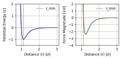
The Lennard-Jones potential (as shown in Fig. Fig. 2.2) is incredibly popular for a whole range of models and is frequently used across fields. It can be used to model simple model liquid systems, predict phase diagrams, and much more.

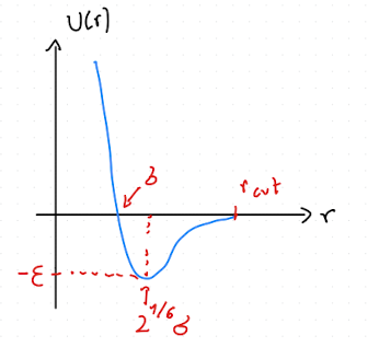
Fig. 2.2 Lennard-Jones potential \(U(r)\) as function of distance \(r\). Here, \(\sigma\) corresponds to a particle size, and \(-\varepsilon\) is the interaction energy at the minimum of the potential, which is located at \(r=2^{1/6}\sigma\).

It is helpful to plot these non-bonded interaction potentials with python and matplotlib, vary the parameters to familiarize ourselves with the shapes and the effects of each parameter.

2.2.4. Total potential energy

The total potential engery is the sum of all one-body, two-body, and higher-body interactions. One-body interactions are for example caused by external fields or forces. Two body interactions are interactions as described above.

\( U = \sum_i u(r_i) + \sum_i \sum_{j>i} u(r_i,r_j) + \sum_i \sum_{j>i} \sum_{k>j} u(r_i,r_j,r_k)+ \ldots \)

2.2.5. Two-Body Approximation

Three-body (and higher) forces are expensive to compute (combinatorics!). Usually, we truncate at two-body interactions and use an effective potential (Fig. 2.3), that reproduces relevant properties.

Other forces (e.g., polar forces) are often neglected.

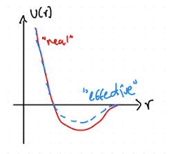
Fig. 2.3 “Effective” pair potential that incoperates some approximation of three-body effects.

Atomistic force fields often consists of two-body non-bonded interactions, bonds, angles and dihedrals.

2.2.5.1. Many-Body Potentials

The overall potential is can be expressed as a series of one-body, two-body, three-body, and higher order potentials.

\[ V=\sum_{i} V_{1}\left(r_{i}\right)+\sum_{i, j} V_{2}\left(r_{i j}\right)+\sum_{i, j, k} V_{3}\left(r_{i j}, r_{i k}, r_{j k}\right)+\cdots \]

The embedded atom method adds a potential term for each atom that is a function of the local density \(\rho_{i}\) around the atom,

\[\begin{split} V=\sum_{i<j} V_{2}\left(r_{i j}\right)+\sum_{i} F\left(\rho_{i}\right) \\ \rho_{i}=\sum_{j} f\left(r_{i j}\right) \end{split}\]

\(F(r)\) and \(f(r)\) are empirical functions defined by these equations.

Example: Stillinger-Weber potential for silicon

The Stillinger-Weber potential for silicon has a three-body term that encourages tetragonal bond angles,

\[\begin{split} V_{2}(r) & =\left(\frac{B}{r^{4}}-A\right) e^{\frac{1}{r-a}} \\ V_{3}\left(r_{i j}, r_{i k}, \theta_{j i k}\right) & =\lambda e^{\frac{\gamma}{r_{i j}-a}+\frac{\gamma}{r_{i j}-a}}\left[\cos (\theta)+\frac{1}{3}\right]^{2} \end{split}\]

where \(\theta_{j i k}\) is the angle between \(\mathbf{r}_{i j}\) and \(\mathbf{r}_{i k}\). These potential functions are set to zero for \(r>a=\) \(3.77 \mathring{A}\).

2.2.6. Coarse-Grained Models

• Atomistic resolution may be impractical for large systems.

Example: Nanoparticles in Water

1 water molecule ≈ 3 Å, 1 nanoparticle ≈ 10 nm results in 1 NP diameter ≈ 30 water molecules. If we compare volume \(V_{np}=\frac{4\pi}{3}(5\text{nm})^3\), then we need \(\sim 37,000\) water molecules to fill the same space as one nanoparticle. If, additionally, we are interested in dilute situations, the vast majority of the system is comprised of the solvent.

In these cases, we study models of the particles we care about with effective interactions that coarsen out the pieces of the system we do not care about, i.e the solvent, as illustrated in Fig. 2.4.

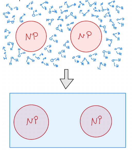
Fig. 2.4 Illustration of coarse-graining by removing solvent. The top shows so-called explicit solvent, e.g. water molecules, and the bottom panel shows the same system where the solvent is replaced with a homogenous “background” that is treated implicitly by modifing the pair interactions. This is called a implicit solvent model.

Coarse-graining removes degrees of freedom and is therefore less accurate, and often considered a empirical approach.

• How to get these effective interactions:

  • Force matching

  • Relative entropy minimization

  • Inverse Boltzmann iteration

2.2.6.1. Simple Examples for coarse-grained Models

Even though a coarse-grained or simplified model lost some amout of detail and degrees of freedom, they often offer a lot of insights.

• Hard spheres: \( u(r) = \begin{cases} \infty & r < d \\ 0 & r \geq d \end{cases} \)

• Lennard-Jones spheres for liquids

• Bead-spring polymers:

  • FENE (Finite Extensible Nonlinear Elastic) Spring model

2.2.7. Force Fields

• Parametrized, self-consistent models fit to thermodynamic or structural data.

• Designed for specific systems:

  • OPLS⁷: hydrocarbons

  • SPC/E, TIP4P/2005, OPC, …:²⁰ water models

  • AMBER, CHARMM: biomolecules

  • TraPPE: phase equilibrium

  • Martini¹⁶: coarse-grained lipids and biomolecules in water

• Machine Learning (ML) models trained on quantum mechanics data are becoming popular.

• You can create or refit your own force field, however validation is crucial.

• How to get the parameters and functional forms for these force fields:

  • experimental information to parameterize model parameters

  • ab-initio calculations from Density Functional Theory (DFT) or other quantum methods

2.2.8. Reduced Units

• SI units are too small and often inconvinient for atomic systems.

• Use reduced units where quantities are of order 1. This also helps with numerical stability and readability of simulation code.

2.2.8.1. Unit Systems

Traditional unit systems can be looked at as follows:

Quantity	SI	CGS	Imperial
length	m	cm	ft
mass	kg	g	lb
time	s	s	s

Other units follow from the base units defined abve in the table.

Example: Unit Consistency

Energy: \( E = \frac{[\text{mass}] [\text{length}]^2}{[\text{time}]^2} = \frac{m l^2 }{ t^2} \rightarrow J = \frac{kg \cdot m^2}{s^2}\) ✅

• For reduced units, choose \( l, m, E \) based on the problem:

  • \(l = \) length = diameter of atom (LJ \(\sigma\), Å)

  • \( m = \) mass = mass of atom (10s amu)

  • \( E = \) energy = interaction energy or thermal energy at reference temperature (\(k_B T\)) (LJ \(\varepsilon\))

This then leads to derived units from your base reduced units:

Derived unit	Relation to base units
area	\([\mathrm{length}]^2\)
volume	\([\mathrm{length}]^3\)
time	\([\mathrm{energy}]^{-1/2} \cdot [\mathrm{length}] \cdot [\mathrm{mass}]^{1/2}\)
velocity	\([\mathrm{energy}]^{1/2} \cdot [\mathrm{mass}]^{-1/2}\)
force	\([\mathrm{energy}] \cdot [\mathrm{length}]^{-1}\)
pressure	\([\mathrm{energy}] \cdot [\mathrm{length}]^{-3}\)
charge	\(`\left(4 \pi \epsilon_{0} \cdot [\mathrm{energy}] \cdot [\mathrm{length}] \right)^{1/2}\)

Here, \(\epsilon_{0}\) is permittivity of free space.

Note that for example time, often called \(\tau\), is a derived unit in reduced unit systems, where it is a base unit in traditional unit systems. We can do that because we can choose \( l, m, E \) sutiable for the system of interest.

2.2.8.2. GROMACS Units

Quantity		Unit
Length	\(l\)	nm
Mass	\(m\)	amu (g/mol)
Energy	\(\varepsilon\)	kJ/mol
Charge	\(q\)	e (\(=1.602 \cdot 10^{-19}\) coulombs)

Quantity		Derived Unit
Time	\(\tau = \sqrt{\frac{m \cdot \sigma^2 }{ \varepsilon}}\)	ps
Velocity	\(l/\tau\)	nm/ps
Force	\(\varepsilon/l\)	kJ/mol/nm
Pressure	\(\varepsilon/l^3\)	kJ/mol/nm³
Viscosity	\(\varepsilon \tau/l^3\)	kJ/mol·ps/nm³
Diffusivity	\(l^2/\tau\)	nm²/ps

• Temperature is either in its own units or derived via Boltzmann constant: \( T = \frac{E}{k_B} \)

Example: Time Units

Time in reduced units: \( \tau = \sqrt{\frac{[\text{mass}] [\text{length}]^2 }{ [\text{energy}]}} \rightarrow \tau = \sqrt{\frac{m \cdot \sigma^2 }{ \varepsilon}}\).

Time in GROMACS units: \(\tau = \sqrt{(10^{-3}kg/mol\cdot (10^{-9}m)^2)/(10^3 J/mol)} = 10^{-12}s\) = ps. ✅

2.2.8.3. LAMMPS Units

LAMMPS offers many different unit systems to use.

Warning

Simulation software may use inconsistent units (e.g., LAMMPS “real” units). Always convert carefully.

Arbitrary units are useful for generalizing results to new problems →Corresponding states principle.

2.2.9. References

• Allen & Tildesley, “Simulations of liquids” Appendix B - Reduced Units ¹

• “Understanding three-body contributions to coarse-grained force fields” Christoph Scherer and Denis Andrienko Phys. Chem. Chem. Phys., 2018,20, 22387-22394¹⁴

• “Effective Two-Body Interactions” Cameron Mackie, Alexander Zech, Martin Head-Gordon, J. Phys. Chem. A 2021, 125, 35, 7750–7758¹⁰

• Force Fields in GROMACS