2.6. Long-Range Potentials

Decay is slower than \(r^{-d}\), where \( d\) is dimensionality.

Note

The formal definition is given over the integral

\[\begin{align*} I = \int_R^D d^D r \frac{A}{r^n} = \begin{cases} \infty &\text{ for } n \leq D \\ \text{finite} &\text{ for } n > D \end{cases} \end{align*}\]

where \(D\) is the dimension. I.e we look at the potential \(u(r)\) as \(r \rightarrow \infty\). This integral then contains \(\frac{r^{D-1}}{r^n}\). In 3D, a potential is short-ranged if it converges faster than \(r^{-3}\). In 2D, a potential is short-ranged if it converges faster than \(r^{-2}\).

Coulomb potential for charges:

\[\begin{align*} u(r) = \frac{q_i q_j}{4\pi \varepsilon_0 r} \end{align*}\]

where \(q_i,q_j\) are the charges, and \(\varepsilon_0\) is the permittivity of free space. Sometimes the factor of \(4\pi\) is not written.

Other long range forces include dipoles, low Reynolds number hydrodynamics, etc.

Interaction can extend much further than the simulation box. How to deal with this?

• Use a bigger box (expensive!)

• Include more than one image of each particle in the calculation

2.6.1. Electrostatics

Most common example for long-range potentials that need to be considered in particle based simulations.

2.6.2. Ewald Sums

• Developed by Ewald (1921), Madelung (1918)

For the calculation of the electric potential \(U\) of an ion at position \(r_i\) due to all other ions of the lattice, we need to compute a sum like this:

\[\begin{align*} U = \frac{1}{2} \sum_{\vec{m}\in \mathbb{Z}^3} \sum_{j}^N \sum_{j \neq i}^N \frac{q_i q_j}{4 \pi \epsilon_0 |\mathbf{r}_i - \mathbf{r}_j + \vec{m}L|} \end{align*}\]

where \(\vec{m}\) are the image vectors, and \(L\) is the box size.

This sum is conditionally convergent!

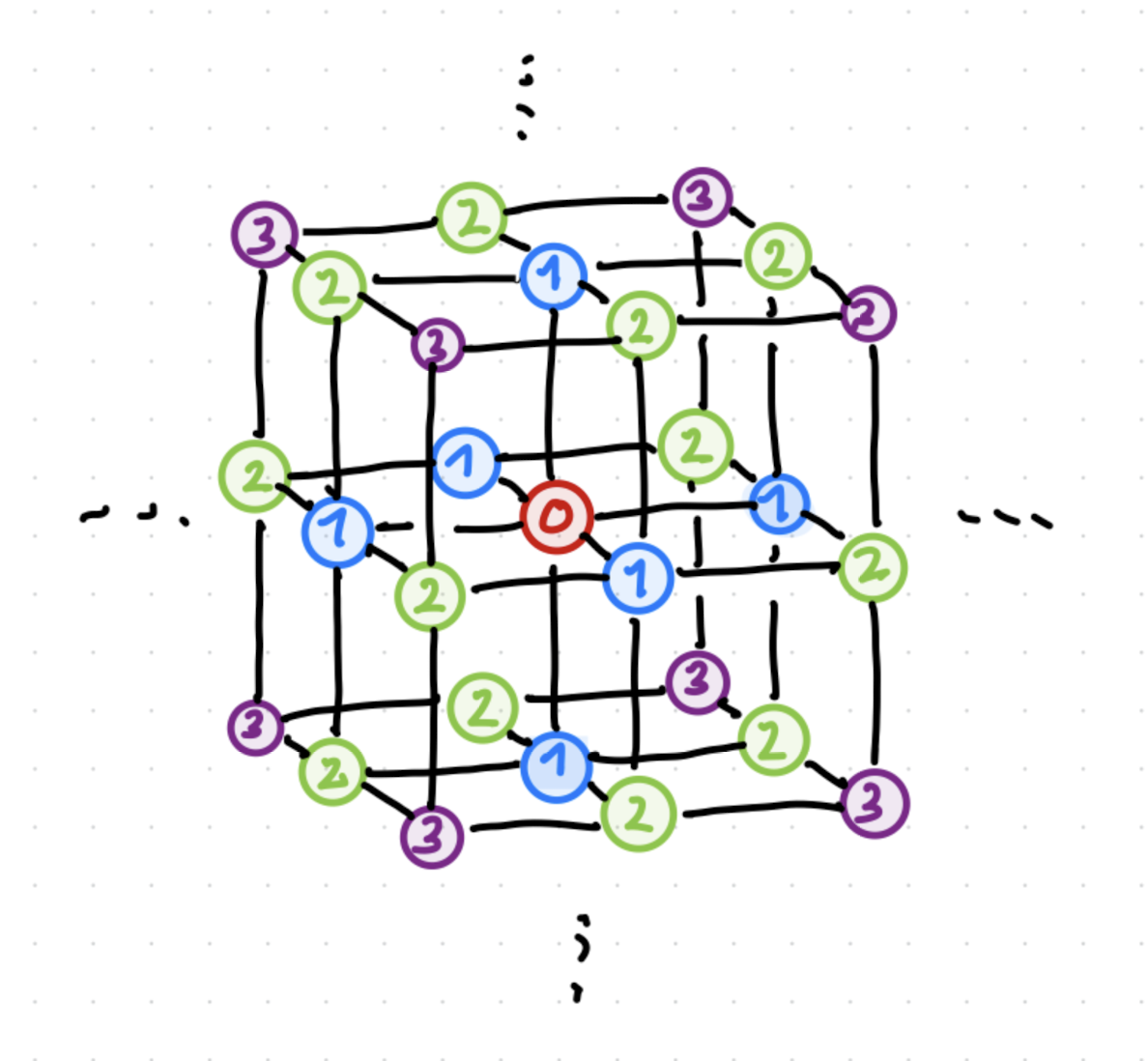
Fig. 2.18 Illustration of the summation of charges on a simple lattice (NaCl). The particle in the center, \(0\), indicates \(i\), and the others are labeled by a possible order of how they could be summed.

Fig. 2.18 shows a simple NaCl crystal. Here, the nearest neighbors contribute \(-\frac{e^2}{4\pi\epsilon_0}\frac{6}{a}\), then the second nearest neighbors contribute \(+\frac{e^2}{4\pi\epsilon_0}\frac{12}{a\sqrt{2}}\), the third \(-\frac{e^2}{4\pi\epsilon_0}\frac{8}{a\sqrt{3}}\), and so on. This doesn’t obviously converge without some math tricks and rearanging. This general challenge exist for any system with long range interactions, in various lattice tpyes.

Solution: Add and subtract a Gaussian charge at each point charge source:

• Point charge:\( \rho(\vec{r}) = q_i\delta(\vec{r}-\vec{r}_i)\)

• Gaussian:\( \rho(\vec{r})^G = \frac{q_i}{(2 \pi \sigma^2)^{3/2}} e^{-|\vec{r}-\vec{r}_i|^2/2\sigma^2}\). Note that \(\rho(\vec{r})^G \rightarrow \rho(\vec{r})\) as \(\sigma \rightarrow 0\).

This scheme is illustrated in Fig. 2.19.

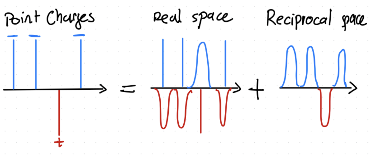
Fig. 2.19 Illustration of the summation of charges on a simple lattice (NaCl). The particle in the center, \(0\), indicates \(i\), and the others are labeled by a possible order of how they could be summed.

How Does This Help?

• The Gaussian charge screens the point charge, making the sum converge faster.

• The cancelling Gaussian charge can also be summed.

• The problem is therefore split into two solvable parts.

For doing this, we do need the electric potential of a Gaussian charge. We use Poisson’s equation

\[\begin{align*} \Delta \phi^G = \nabla^2 \varphi^G &= - \frac{\rho^G}{\epsilon_0}\\ \frac{1}{r} \frac{d^2(r \phi^G)}{dr^2} &= -\frac{q_i}{\epsilon_0(2 \pi \sigma^2)^{3/2}} e^{-r^2/2\sigma^2}\\ \int_\infty^r dr \frac{d^2(r \phi^G)}{dr^2} &= \int_\infty^r dr \left[-\frac{q_i r }{\epsilon_0(2 \pi \sigma^2)^{3/2}} \right] e^{-r^2/2\sigma^2}\\ \frac{d(r \phi^G)}{dr} &= \frac{\sigma^2}{\epsilon_0}\frac{q_i}{(2 \pi \sigma^2)^{3/2}} e^{-r^2/2\sigma^2}\\ \int_0^r d(r \phi^G) &= \frac{q_i\sigma^2}{\epsilon_0}\frac{1}{(2 \pi \sigma^2)^{3/2}} \int_0^r dr e^{-r^2/2\sigma^2}\\ \dots \rightarrow \phi^G &= \frac{q_i}{4\pi\epsilon_0r} \mathrm{erf}(\frac{r}{\sqrt{2}\sigma}) \quad . \end{align*}\]

For a simple point charge, we get

\[\begin{align*} \phi(r) = \frac{q_i}{4\pi\epsilon_0 r} \quad . \end{align*}\]

Using this, we can split the sum, called Ewald summation, which we will derive below.

\[\begin{align*} \phi(\vec{r})&=\frac{1}{4 \pi \varepsilon_0} \sum_\vec{m} \sum_{j=1}^N \frac{q_j}{|\vec{r}_i \vec{r}+\vec{m}L|}\\ \rightarrow u&=\frac{1}{2} \sum_{i=1}^N q_i[\phi(\vec{r}_i)-\underbrace{\phi_i(r_i)}_{\substack{\text{exclude self interactions}\\ \text{where } \vec{m}=0}}] \end{align*}\]

Note

We exclude self-interactions, but they can be kept in principle. In the final equation in the summary below, we list them explicitly, but commonly they are exlcuded or set to zero.

Now we split the sum:

\[\begin{align*} \phi_i(r) &= \underbrace{\phi_i(r)-\phi^G_i(r)}_{\text{short}} + \underbrace{\phi^G_i(r)}_{\text{long}}\\ & =\frac{q_i}{4 \pi \epsilon_0 r}-\frac{q_i}{4 \pi \epsilon_0 r} \operatorname{erf}\left(\frac{r}{\sqrt{2} \sigma}\right)+\frac{q_i}{4 \pi \varepsilon_0 r} \operatorname{erf}\left(\frac{r}{\sqrt{2} \sigma}\right) \\ & =\frac{q_i}{4 \pi \varepsilon_0 r}\left[1-\operatorname{erf}\left(\frac{r}{\sqrt{2} \sigma}\right)\right]+\frac{q_i}{4 \pi \varepsilon_0 r} \operatorname{erf}\left(\frac{r}{\sqrt{2} \sigma}\right) \\ & =\frac{q_i}{4 \pi \varepsilon_0 r} \operatorname{erfc}\left(\frac{r}{\sqrt{2} \sigma}\right)+\frac{q_i}{4 \pi \varepsilon_0 r} \operatorname{erf}\left(\frac{r}{\sqrt{2} \sigma}\right)\\ & =\frac{q_i}{4 \pi \varepsilon_0 r} \operatorname{erfc}\left(\kappa r \right)+\frac{q_i}{4 \pi \varepsilon_0 r} \operatorname{erf}\left(\kappa r\right) \end{align*}\]

Where we have defined an inverse screening length \(\kappa = \frac{1}{\sqrt{2}\sigma}\) in the last step.

Now we define a short ranged \(\phi_i^S(r)\) and a long ranged \(\phi_i^L(r)\),

\[\begin{align*} \phi_i^S(r)=\frac{q_i}{4 \pi \varepsilon_0 r} \operatorname{erfc}\left(\frac{r}{\sqrt{2} \sigma}\right) \\ \phi_i^L(r)=\frac{q_i}{4 \pi \varepsilon_0 r} \operatorname{erf}\left(\frac{r}{\sqrt{2} \sigma}\right) \end{align*}\]

so that we get

\[\begin{align*} \phi(r)&=\sum_\vec{m} \sum_{j=1}^N \phi_j\left(\left|\vec{r}_i-\vec{r}+\vec{m} L\right|\right) \\ & =\sum_\vec{m} \sum_{j=1}^N \phi_j^S+\phi_j^L\\ &=\sum_\vec{m} \sum_{j=1}^N \phi_j^S+\sum_\vec{m} \sum_{j=1}^N\phi_j^L\\ &=\phi^S+\phi^L \quad , \\ \end{align*}\]

and

\[\begin{align*} u&=\frac{1}{2} \sum_{i=1}^N q_i\left[\phi^S\left(r_i\right)-\phi_i^S\left(r_i\right)\right]+\frac{1}{2} \sum_{i=1}^N q_i\left[\phi^L\left(r_i\right)-\phi_i^L\left(r_i\right)\right] \\ &=\frac{1}{2} \sum_\vec{m} \sum_{i=1}^N \sum_{j=1, i\neq j}^N u^S\left(\left|r_j-r_i+\vec{m}L\right|\right)+\frac{1}{2} \sum_{i=1}^N q_i \phi^L\left(r_i\right)-\frac{1}{2} \sum_{i=1}^N q_i \phi_i^L\left(r_i\right) \\ \end{align*}\]

For the last sum, we can now look at the limit:

\[\begin{align*} \lim_{r \rightarrow 0} \frac{q_i}{4 \pi \varepsilon_i r} \operatorname{erf}\left(\frac{r}{\sqrt{2} \sigma}\right)= \frac{q_i}{4 \pi \varepsilon_i} \frac{1}{\sigma} \sqrt{\frac{2}{\pi}} \end{align*}\]

This results in

\[\begin{align*} u&=\underbrace{\frac{1}{2} \sum_\vec{m} \sum_{i=1}^N \sum_{j=1, i\neq j}^N u^S\left(\left|r_j-r_i+\vec{m}L\right|\right)}_{u^S(r)=\frac{q_iq_j}{4\pi\varepsilon_0r}\operatorname{erfc}\left(\frac{r}{\sqrt{2}\sigma}\right)}+ \frac{1}{2} \sum_{i=1}^N q_i \phi^L\left(r_i\right) -\frac{1}{4 \pi \varepsilon_0} \frac{1}{\sqrt{2}\sigma} \frac{1}{\sqrt{\pi}} \sum_{i=1}^N q_i^2 \end{align*}\]

The first term, turns into a normal pairwise sum, if \(\operatorname{erfc}\) decays quickly. The middle term still needs to be evaluated.

Long-ranged part is convieniently summed in Fourier space. Fourier transform:

\[\begin{align*} \hat f(\vec{k}) &= \int_V d\vec{r} f(\vec{r}) e^{-i\vec{k}\vec{r}} \quad \text{for finite volumes. }\\ \hat f(\vec{r}) &= \frac{1}{L^3} \sum_\vec{k} \hat f(\vec{k}) e^{i\vec{k}\vec{r}} \quad \text{with } \vec{k} = \frac{2\pi \vec{n}}{L} \quad . \end{align*}\]

We need to Fourier transform Poisson’s equation for Gaussian charge (periodic array).

\[\begin{align*} & \nabla^2 \phi^G=-\frac{\rho^G}{\varepsilon_0} \rightarrow -k^2 \hat{\phi}^G=-\frac{\hat{\rho}^G}{\varepsilon_0} \rightarrow \hat{\phi}^G=\frac{1}{k^2 \varepsilon_0} \hat{\rho}^G \end{align*}\]

Now we can compute

\[\begin{align*} & \hat{\rho}^G(\vec{k})=\int_V dr -\frac{q_i}{\left(2 \pi \sigma^2\right)^{3 / 2}} e^{-\left|\vec{r}-\vec{r}_i+\vec{m}L\right|^2 / 2 \sigma^2} e^{-i \vec{k} \cdot \vec{r}} \\ & =-\int dr \frac{q_i}{\left(2 \pi \sigma^2\right)^{3 / 2}} e^{-\left|\vec{r}-\vec{r}_i\right|^2 / 2 \sigma^2} e^{-i \vec{k} \cdot \vec{r}} \\ \end{align*}\]

where we used the fact that the shifts (\vec{m}) add up to infinite space and we can convert the integral.

\[\begin{align*} & =\int d r \frac{q_i}{\left(2 \pi \sigma^2\right)^{3 / 2}} e^{-r^2 / 2 \sigma^2} e^{-i \vec{k} \cdot\left(\vec{r}+\vec{r}_i\right)} \\ & =e^{-i \vec{k} \cdot \vec{r}_i} \int_0^{\infty} dr r^2 \int_0^{2 \pi} d\theta \int_{-1}^1 d \cos \phi \frac{q_i}{\left(2 \pi \sigma^2\right)^{3 / 2}} e^{-r^2 / 2 \sigma^2} e^{-i k r \cos \phi} \end{align*}\]

The integration here got changed to spherical coordinates.

\[\begin{align*} \dots \end{align*}\]

Hence, \(\hat{\phi}_i^G(k)=\frac{q_i}{\varepsilon_0 k^2} e^{-k^2 \sigma^2 / 2} e^{-i \vec{k} \cdot \vec{r}_i}\).

Last, invert

\[\begin{align*} \phi^L(\vec{r}) & =\frac{1}{L^3} \sum_\vec{k} \hat{\phi}(\vec{k}) e^{i \vec{k} \cdot \vec{r}} \\ & =\frac{1}{L^3} \sum_{\vec{k} \neq 0} \frac{q_j}{\varepsilon_0 k^2} e^{-k^2 \sigma^2 / 2} e^{-i \vec{k} \cdot\left(\vec{r}_j-\vec{r}\right)} \end{align*}\]

and

\[\begin{align*} U^L=\frac{1}{2} \sum_{i=1}^N \sum_{i=1}^N \sum_{\vec{k} \neq 0} \frac{q_i q_i}{\varepsilon_0 k^2 L^3} e^{-k^2 \sigma^2 / 2} e^{-i \vec{k} \cdot \vec{r}_{i j}} \quad . \end{align*}\]

2.6.2.1. Boundary Effects

The lattice needs to be truncated somewhere, so it is effectively embedded in som medium. At this boundary, there is a depolarizing field counteracting the fluctuatin dipole moment of the main cell.

\[\begin{align*} U^{BC} = \frac{1}{2(2\varepsilon_r+1)\varepsilon_0 L^3} |\sum_{i=1}^N q_i r_i|^2 \end{align*}\]

For so called “tin foil” BCs used in most simulations, set \(\varepsilon_r=\infty\).

2.6.2.2. Summary

In summary,

\[\begin{align*} u &=\underbrace{\frac{1}{2} \sum_\vec{m} \sum_{i=1}^N \sum_{i=1, i\neq j}^N \frac{q_i q_i}{4 \pi \varepsilon_0\left|r_{i j}+mL\right|} \operatorname{erfc}\left(\kappa | r_{ij}+m L|\right)}_{\text{short}} \\ & \underbrace{+\frac{1}{2} \sum_{\vec{k} \neq 0} \sum_{i=1}^N \sum_{j=1}^N \frac{q_i q_j}{\varepsilon_0 k^2 L^3} e^{-k^2 / 4 \kappa^2} e^{-i \vec{k} \cdot \vec{r}_{ij}}}_{\text{long}} \\ & \underbrace{-\frac{\kappa}{4 \pi^{3 / 2} \varepsilon_0} \sum_{i=1}^N q_i^2}_{\text{self}} \\ & \underbrace{+\frac{1}{2\left(2 \varepsilon_r+1\right) \varepsilon_0 L^3}\left|\sum_{i=1}^N q_i \vec{r}_i\right|^2}_{\text{BC}} \end{align*}\]

• Real space: efficient for short-range potentials

• Reciprocal space: efficient way to treat smooth periodic functions

• Ewald: efficient way to sum a divergent and long-range interaction by summing part in real space and part in reciprocal space

Choose \(k=\frac{1}{\sqrt{2}\sigma}\), the inverse screening length, and the number of wavevectors to be accurate and efficient.

• Self-interactions are commonly excluded.

2.6.3. Alternative Methods

• Direct summation, Laplace, 1820, \(\mathcal{O}(N^2)\)

• Ewald summation, Ewald, 1921 (with adjusted E and neighbor tables) \(\mathcal{O}(N^{3/2})\)

• Multigrid summation, Brandt, 1977, \(\mathcal{O}(N)\)

• Barnes-Hut Treecode, Barnes, Hut, 1986, \(\mathcal{O}(N \log N)\)

• Fast Multipole Method, Greengard, Rokhlin, 1987, \(\mathcal{O}(N)\)

• Particle-Particle Particle-Mesh, Hockney, Eastwood, 1988,\(\mathcal{O}(N \log N)\)

• Particle Mesh Ewald, Darden, 1993, \(\mathcal{O}(N \log N)\)

2.6.4. Additional Resources

• “On mesh-based Ewald methods: Optimal parameters for two differentiation schemes” Harry A. Stern; Keith G. Calkins J. Chem. Phys. 128, 214106 (2008)

• Shape-Adapted Ewald Summation, M. Widom