2.3. Periodic Boundary Conditions#
2.3.1. Studying “real” systems with small simulations#
Simulations can usually only handle \( N \approx 10^4 - 10^6 \) particles (routinely) because:
Model gets too big for computer memory
Time to run simulation gets too long
“Real” systems have moles \( N \sim 10^{23} \) worth of particles!
\(\rightarrow\) Can a smaller simulation capture this?
2.3.1.1. Challenge: Surface-to-volume ratio#
Surfaces often lead to different behavior than bulk.
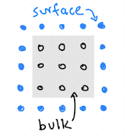
Fig. 2.5 2D Visualization of surface vs. bulk in a simple lattice system. Only 9 particles are in the “bulk” and 16 are on the surface.#
\( N = L^3 \) particles on a cubic lattice
\( N_{\text{bulk}} = (L - 2)^3 \) assuming one particle thick surface on each side
\( N_{\text{surf}} = N - N_{\text{bulk}} = L^3 - (L-2)^3 = 6L^2 - 12L + 8 \)
Fraction of surface particles:
For \( L = 10 \), so \( N = 10^3 \rightarrow N_{\text{surf}} / N \approx 49\% \)
For \( L = 100 \), so \( N = 10^6 \rightarrow N_{\text{surf}} / N \approx 6\% \)
Measurements will include significant surface contributions that deviate from “bulk”, especially for “small” systems. These deviations from the bulk, or the thermodynamic (\(L \rightarrow \infty\)) limit are often called finite size effects.
Consider a drop of \(N\) atoms in free space. (For example a galaxy, a protein in vacuum, or a droplet) How many are on the surface and how does that converge in \(N\)? The fraction of surface atoms is proportional to \(N^-1/3\). If the droplet contains one million atoms and the surface layer is only 5 atoms deep, 25% of atoms are still on the surface! This is not a very efficient way of sampling a bulk system. There are other problems as well. With free boundary conditions one can only do simulations at zero pressure and there is nothing to keep the atoms from evaporating. Also the equilibration time can be much longer than it bulk since surface process can be much slower.
2.3.2. Definiton of Periodic Boundary Conditions#
Embed the simulated system in an “infinite” one made by copying it. This works with all box shapes that can be tiled in space.
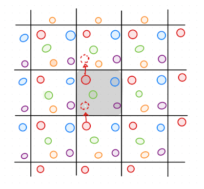
Fig. 2.6 Visualization of periodically copying a system to make it “infinite”.#
There are no surfaces!
Only capture one subsystem (the one marked in light gray in Fig. 2.6), then copy it.
Can use any space-filling box shape, but most common is a parallelepiped (or special cases like rectangular prism or cube), as shown in Fig. 2.7.
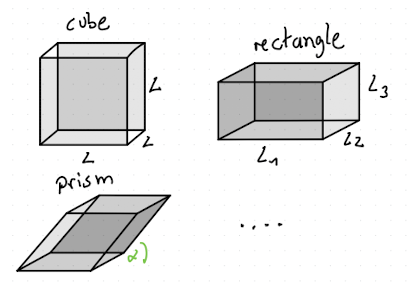
Fig. 2.7 isualization of different simulation box shapes.#
An alternative way to look at it is to “wrap” the simulation volume, as shown in Fig. 2.8.
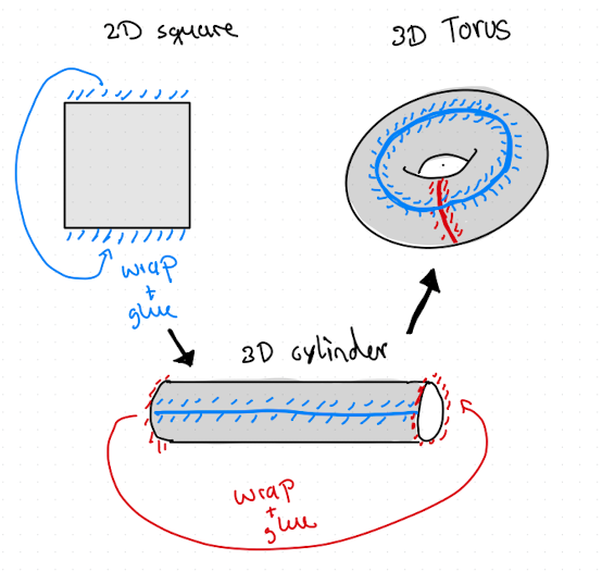
Fig. 2.8 Visualization of periodic “wrapping” of the edges of a simulation box in higer dimension to elimiate surfaces/edges.#
How does this help?
Only track particles in the volume of interest (images replace each other when they enter/leave).
If model potentials are short-ranged, only compute over a small volume of the “infinite” system. Hence, you can model bulk thermodynamic behavior using a nanoscopic volume.
It has been found that hundreds of atoms in PBC can behave like an infinite system in many respects. The finite size corrections are order \((1/N)\) and the coefficient can be small. One cannot calculate long distance behavior \((~L/2)\). Angular momentum might no longer be conserved in a finite system. Also PBC can influence the stability of phases. For example, PBC favor cubic lattice structures that fit well into the box.
Alternative Boundaries
Simulations on a sphere surface: The geometry is non-Cartesian (there is a curvature to space) and calculating distances is more complicated. The representation of crystals is a problem since there are only 5 perfect lattices on a sphere with 4, 6, 8 12 and 20 particles.
External “wall” potentials: An example would be a liquid in a tube (cylindrical confinement), spherical confinement, slab geometry (two PBC directions, one direction with a flat wall), etc.
2.3.3. Implementation of Periodic Boundary Conditions#
2.3.3.1. Particle Wrapping#
When a particle leaves, \(x\), one of its images enters. Wrapping computes this position \(x'\), as show in Fig. 2.9.
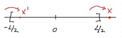
Fig. 2.9 Position \(x\) of particle in 1D periodic system of size \(L\).#
Note
Defintion of the domain (or box origin) is flexible. Common conventions include \(-L/2\leq x \le L/2\) and \(0\leq x \le L\). Different codes and open source packages might use different conventions.
One way to compute the positions:
if x = L/2 , then  x' = x - L
else if  x < -L/2 , then  x' = x + L
Example: PBC
If box is \(L=10\), all positions need to be between \(-5\) and \(5\). If \(x=6\), we need to wrap:
\(L = 10 \), \( x = 6 \rightarrow x' = 6 - 10 = -4 \) ✅
What if \( x \) lies far away, i.e much larger/smaller than L??
Use while loops:
x' = x
while x' > L/2: x' = x' - L
while x' < -L/2: x' = x' + L
Example: PBC using while
\(x = 16 \rightarrow x' = 6 \rightarrow x'=-4 \) ✅
More efficient way is to use nearest integer rounding to compute number of interations. The nearest integer value can be tracked and used to unwrap and wrap trajectories for visualizations or calculations.
n = round(x/L)
x' = x - n*L
Example: PBC using round
\(n = \text{round}(16/10) = \text{round}(1.6) = 2\)
\( x' = 16 - 2\cdot(10) = -4 \) ✅
2.3.3.2. Minimum Image Convention#
How to find the image that is closest to a particle? This is needed for example for force calculations.
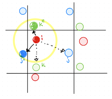
Fig. 2.10 Illustration of the minimum image convention. Particles within the yellow circle are closer to each other, even though they are in the “copied” systems, i.e the solid arrows indicate the shortest distances, rather than the “naively computed” dashed distances.#
As shown in Fig. 2.10, particles in the “copied” or tiled systems can be closer to a particle than the particle in the original box.
The same code and ideas presented in the section above works on distance vectors \(\vec r_{ij}= \vec r_i - \vec r_j\) (as defined in the original box):
\(\vec r_{ij}' = \vec r_{ij} - L\cdot\text{round}( \vec r_{ij}/L)\).
Warning
Do not look further than \(r =L/2\), or additional further out images could be needed. This is generally not advisable.
As a rule of thumb: A simulation box should be at least twice as large than the longest interaction range to avoid issues where particles might interact with their own images, which is unphysical.
2.3.4. Some Caveats to be aware of when using Periodic Boundary Conditions#
Waves:
PBCs restricht the waves that fit into a simulation box, since they must have a compatible wavelength, as illustrated in Fig. 2.11.
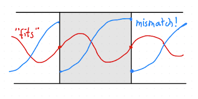
Fig. 2.11 Certain wavelengths are restricted in periodic boxes, since they need to be compatible with the box dimensions.#
The condition is that \(k = \frac{2\pi n}{L}\), with \(n\) being integers. This means that longer wavelengths might be suppressed in smaller boxes, and may impact properties, for example:
large fluctuations near a critial point \(\rightarrow\) the value of the critical temperature \(T_c\) measured in the simulation depends on system size
interfacial tensions \(\gamma\) depend strongly on the waves that exist on the surface,so measured values of \(\gamma\) will be influenced by system size
…
Periodicity:
Any structure in the simulation must be compatible with the PBCs, and, effectively, becomes periodic on lengths \(L\).
for solids, one needs to make sure that the box matches the crystal lattice (both for dimensions and angles/orientation)
for periodic structures like lamellae, membranes, etc., similar arguments apply
This may impact properties measured, if the box is slightly off the “preferred” dimensions.
Finite size effects:
Some properties that are computed, including phase transions and diffusion constants, interfacial tensions, etc. will depend on \(L\). These can oftem be systematically corrected by doing a finite size study, that involves measuring the quantities of interest in various box sizes, plotting them as function of \(1/L\) (or other theoretically known scaling) and then extrapolating to the thermodynamic limit: \(L \rightarrow \infty \Rightarrow 1/L \rightarrow 0\).
Note
It is always a good idea to test these effects by running some extra simulations in bigger and smaller boxes to assess if/how much results change.
A longer chapter on finite size effects from the perspecitive of phase transitions and critical points is in the Monte-Carlo section of this book.
2.3.5. Additional Resorces#
“A Guide to Monte Carlo Simulations in Statistical Physics”,Landau, Binder{cite:landau2021guide} has extensive theoretical explanations and details about finite size effects.