2.4. Intermolecular Potentials

in Fig. 2.12 most typical intermolecular potentials for a molecule are shown.

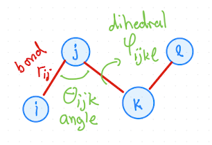
Fig. 2.12 Visualization of bonds, angles, and dihedrals in a molecule with four atoms.

The overall energy is given by:

\[ U = \sum_{\text{bonds}, {i,j} } U_b(r_{ij}) + \sum_{\text{angles}, {i,j,k}} U_\theta(\theta_{ijk}) + \sum_{\text{dihedrals}, {i,j,k,l} } U_\varphi(\varphi_{ijkl}) \]

To compute a conservative force in general: \( \vec{F}_i = -\nabla_i U \) where \(\nabla_i = \frac{\partial}{\partial r_i}\) is the gradient with respect to \(r_i\).

2.4.1. Bond Potentials

As shown in Fig. 2.13, the bond length between particle \(i\) and \(j\) is given by

\( r_{ij} = \| \vec{r}_i - \vec{r}_j \| = \sqrt{(x_j-x_i)^2 + (y_j-y_i)^2 + (z_j-z_i)^2}\).

The bond vector is \( \vec r_{ij} = \vec{r}_i - \vec{r}_j \).

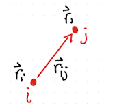
Fig. 2.13 Definition of bond distance.

To obtain the force on a bond we need to compute

\[ F_i = - \nabla_i U_b(r_{ij}) = - \frac{\partial U_b}{\partial r_i} \nabla_i r_{ij}\quad . \]

For this, we need \(\nabla_i r_{ij}\), which is

\[\begin{split} \nabla_i r_{ij} & = \frac{\partial}{\partial x_{i,\alpha}} \left[ \sqrt{(x_{j,\alpha}-x_{i,\alpha})(x_{j,\alpha}-x_{i,\alpha})} \right]\\ & = \frac{1}{2} \frac{-2 x_{j,\alpha}+2x_{i,\alpha}}{\sqrt{(x_{j,\alpha}-x_{i,\alpha})(x_{j,\alpha}-x_{i,\alpha})}}\\ & = - \frac{x_{j,\alpha}-x_{i,\alpha}}{\sqrt{(x_{j,\alpha}-x_{i,\alpha})(x_{j,\alpha}-x_{i,\alpha})}}\\ & = - \frac{r_{ij}}{|r_{ij}|}\\ & = - \hat r_{ij} \end{split}\]

which is the unit vector pointing in the direction of the bond!

The force then is

\[\begin{split} F_i &= - \frac{\partial U_b(r_{ij})}{\delta r_{ij}} (-\hat r_{ij}) \\ &= - F_b(r_{ij}) \hat r_{ij}, \text{ with } F_b(r_{ij}) \equiv - \frac{\partial U_b(r_{ij})}{\delta r_{ij}} \end{split}\]

By symmetry we should have \(\nabla_j r_{ij}=-\nabla_i r_{ji}\), meaning that

\[ F_j = F_b(r_{ij}) \hat r_{ij} \quad. \]

This shows that for a bond, \(F_i = -F_j\), which illustrates that action has a equal and opposite reaction.

Tip

Once can use the action reaction principle to save on computations by only computing either \(F_i\) OR \(F_j\) and then applying the equal action-reaction principle to save on calculations.

2.4.1.1. Harmonic

\( U(r) = \frac{1}{2}k(r - r_0)^2 \)

This fixes the bond length to fluctuate around an average of \(r_0\).

• Watch for factor of 2!

• Typically \( k \sim 10^3 \epsilon/l^2\) for “stiff” bond

Show code cell content

Hide code cell content

from myst_nb import glue
import matplotlib.pyplot as plt
plt.style.use(['../_matplotlib/book.mplstyle'])
import numpy as np

# Harmonic bond potential
def harmonic_bond_potential(r, k, r0):
    return 0.5 * k * (r - r0)**2

# Harmonic bond force
def harmonic_bond_force(r, k, r0):
    return -k * (r - r0)

# Parameters
k = 1.0
r0 = 1.0
r_values = np.linspace(0.5, 1.5, 100)
U_values = harmonic_bond_potential(r_values, k, r0)
F_values = harmonic_bond_force(r_values, k, r0)

fig, axs = plt.subplots(1, 2, figsize=(6,3.5))

axs[0].plot(r_values, U_values,c='lightcoral')
axs[0].axvline(x=r0, linestyle='--',c='dodgerblue', label='$r_0$')
axs[0].set_xlabel('$r$')
axs[0].set_ylabel('$U_{\mathrm{bond}}(r)$')
axs[0].set_title('Harmonic Bond Potential')
axs[0].legend(frameon=False)

axs[1].plot(r_values, F_values,c='seagreen')
axs[1].axvline(x=r0, linestyle='--',c='dodgerblue', label='$r_0$')
axs[1].set_xlabel('$r$')
axs[1].set_ylabel('$F_{\mathrm{bond}}(r)$')
axs[1].set_title('Harmonic Bond Force')
axs[1].legend(frameon=False)

plt.savefig('./_figures/harmonic_bond.png')

<>:26: SyntaxWarning: invalid escape sequence '\m'
<>:33: SyntaxWarning: invalid escape sequence '\m'
<>:26: SyntaxWarning: invalid escape sequence '\m'
<>:33: SyntaxWarning: invalid escape sequence '\m'
/tmp/ipykernel_2205/129747257.py:26: SyntaxWarning: invalid escape sequence '\m'
  axs[0].set_ylabel('$U_{\mathrm{bond}}(r)$')
/tmp/ipykernel_2205/129747257.py:33: SyntaxWarning: invalid escape sequence '\m'
  axs[1].set_ylabel('$F_{\mathrm{bond}}(r)$')

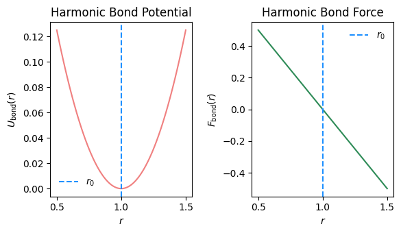
Example: Harmonic bond force

\( U_b = \frac{1}{2}k(r - r_0)^2 \), so

\( F_b = \frac{\partial U_b}{\delta r_{ij}} = -k (r_{ij}-r_0)\), leading to

\[\begin{split} F_i &= + (r_{ij}-r_0) \hat r_{ij}\\ F_j &= - (r_{ij}-r_0) \hat r_{ij} \quad . \end{split}\]

If \(r_{ij}>r_0\), the bond is streched past \(r_0\) and particle \(i\) moves toward \(j\), and \(j\) toward \(i\). If \(r_{ij}<r_0\), the bond is compressed below the set point \(r_0\) and particle \(i\) moves away from \(j\), and \(j\) away from \(i\).

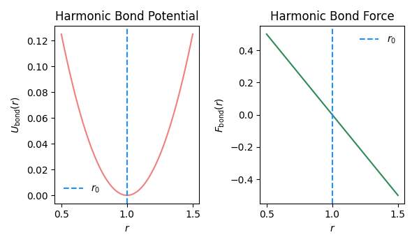
Fig. 2.14 Bond potential and force as function of bond length \(r\).

2.4.1.2. FENE (Finite Extensible Nonlinear Elastic)

\( U(r) = -\frac{1}{2}k r_0^2 \ln\left(1 - \left(\frac{r}{r_0}\right)^2\right) \)

Diverges at \(r_0\), minimum at 0. This is usually used in conjuction with a repulsive, short-ranged force (WCA = cut LJ at minimum and shift up to get a purely repulsive potential).

Typical parameters:

• k = 30, r_0 = 1.5

Show code cell content

Hide code cell content

from myst_nb import glue
import matplotlib.pyplot as plt
plt.style.use(['../_matplotlib/book.mplstyle'])
import numpy as np

# Define parameters for the potentials
k_harmonic = 850.0  # Harmonic bond constant
r0_harmonic = 0.96  # Harmonic equilibrium bond length

k_fene = 30.0      # FENE bond constant
R0_fene = 1.5      # FENE maximum bond extension
epsilon = 1.0
sigma = 1.0

# Define the range of bond distances (r)
r = np.linspace(0.9, 1.1, 500) # Adjust range based on potential parameters

V_harmonic = 0.5 * k_harmonic * (r - r0_harmonic)**2
arg_fene = 1 - (r / R0_fene)**2
V_fene =  -0.5 * k_fene * R0_fene**2 * np.log(arg_fene)

V_fene_wca = V_fene
r_rep = r[r<2**(1/6)]
V_fene_wca[r<2**(1/6)] += 4*epsilon*((sigma/r_rep)**12-(sigma/r_rep)**6)+ epsilon

fig, axs = plt.subplots(1, 1)

axs.plot(r, V_harmonic-np.min(V_harmonic),label='harmonic')
axs.plot(r, V_fene_wca-np.min(V_fene_wca), label='FENE+WCA')
axs.set_xlabel('$r$')
axs.set_ylabel('$U_{\mathrm{bond}}(r)-U_\mathrm{min}$')
axs.legend()

axs.set_ylim(0,6)

plt.savefig('./_figures/FENE_bond.png')

<>:31: SyntaxWarning: invalid escape sequence '\m'
<>:31: SyntaxWarning: invalid escape sequence '\m'
/tmp/ipykernel_2205/912570185.py:31: SyntaxWarning: invalid escape sequence '\m'
  axs.set_ylabel('$U_{\mathrm{bond}}(r)-U_\mathrm{min}$')

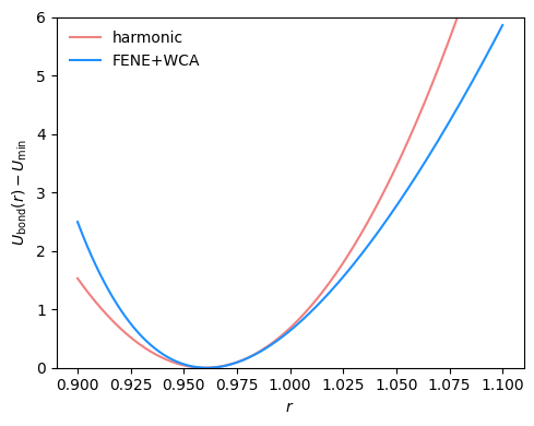
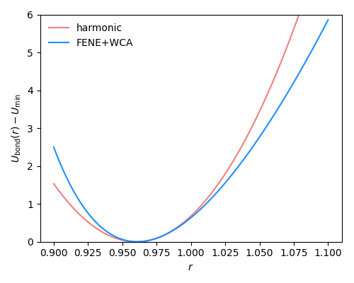
Fig. 2.15 FENE+WCA bond potential with standard parameters \(R_0=1.5\) and \(k=30\) compared to a harmonic bond potential with \(r_0=0.96\) and \(k=850\).

2.4.2. Angle Potentials

The angle between three particles \(i\), \(j\), and \(k\) is given by:

\[ \cos \theta_{ijk} = \frac{(\vec{r}_{ji} \cdot \vec{r}_{jk})}{|\vec{r}_{ji}||\vec{r}_{jk}|} = - \frac{(\vec{r}_{ij} \cdot \vec{r}_{jk})}{|\vec{r}_{ij}||\vec{r}_{jk}|}\quad . \]

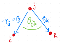
Fig. 2.16 Definition of angle.

Note the negative sign, i.e the two bond vectors point out from the middle particle \(j\).

Note

In polymers, angle θ is sometimes defined as the outer angle. This is less common in atomistic models, but be careful!

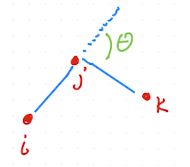
Fig. 2.17 Alternative definition of angle as the outer angle.

These two definitions can be easily converted into each other \(\theta_{ijk} = \pi - \theta'_{ijk}\).

To compute the angle potential between three particles, we need to

\[\begin{split} F_i &= -\nabla_i U_\theta (\theta_{ijk}) \\ &=- \frac{\partial U_\theta}{\partial \theta_{ijk}} \nabla_i \theta_{ijk} \\ \text{ where } - \frac{\partial U_\theta}{\partial \theta_{ijk}} = F_\theta \quad . \end{split}\]

Getting \(\cos^{-1}\) is computationally expensive, which would be needed above. Once can try to avoid that by using the chain rule:

\[\begin{split} F_i &= - \frac{\partial U_\theta}{\partial \theta_{ijk}} \nabla_i \theta_{ijk} \\ F_\theta \frac{\partial \theta_{ijk}}{\partial \cos(\theta_{ijk})} \nabla_i \cos\theta_{ijk} \\ -F_\theta \frac{1}{\sin(\theta_{ijk})} \nabla_i \cos\theta_{ijk}\quad . \end{split}\]

For this, we then need \( \nabla_i \cos\theta_{ijk}\). Eq.7 of J. Chem. Phys. 146, 226101 (2017) offers a compact form.

Warning

\(F_i\) is singlular if \(\theta_{ijk}=0^\circ\) or \(180^\circ\) if \(F_\theta\) is not zero at these points!

2.4.2.1. Harmonic

\[ U_\theta(\theta) = \frac{k}{2} (\theta - \theta_O)^2 \]

Fixes average angle around set point of \(\theta_0\). Like with the harmonic bond potential, whatch for the factor of two in the spring constant.

2.4.2.2. Cosine

\[ U_\theta(\theta) = k (1 + \cos{\theta}) \]

Minimum is when the particles are in colinear \(\theta =180^\circ\) arrangement. There are forms with a set angle different from that, by using \(k (1 - \cos{(\theta - \theta_0)}) \) as functional form.

2.4.2.3. Cosine squared

\[ U_\theta(\theta) = \frac{k}{2} (\cos\theta - \cos\theta_O)^2 \]

Watch out for the exact definition of the parameters, sometimes \(1/2\) is included in the definition of \(k\).

Note

For specific models and force fields, always check if the angles are given in degree or radians.

Show code cell content

Hide code cell content

from myst_nb import glue
import matplotlib.pyplot as plt
plt.style.use(['../_matplotlib/book.mplstyle'])
import numpy as np

# Define the range of angles (in radians)
theta = np.linspace(0, np.pi, 500)  # From 0 to pi radians

# Define potential parameters (example values)
k_harmonic = 1.0  # Force constant for harmonic potential
theta_0_harmonic = np.pi / 2  # Equilibrium angle for harmonic potential

k_cosine = 1.0  # Pre-factor for cosine potential
theta_0_cosine = np.pi / 2 # Equilibrium angle for cosine potential

k_cosine_squared = 1.0  # Pre-factor for cosine-squared potential
theta_0_cosine_squared = np.pi / 2 # Equilibrium angle for cosine-squared potential

# Calculate the potentials
harmonic_potential = 0.5 * k_harmonic * (theta - theta_0_harmonic)**2
cosine_potential = k_cosine * (1 - np.cos(theta - theta_0_cosine)) # Often defined as 1-cos(theta) for a minimum at theta=theta_0
cosine_squared_potential = k_cosine_squared * (1 - np.cos(theta - theta_0_cosine_squared)**2) # Often defined as 1-cos^2(theta) for a minimum at theta=theta_0

# Plotting
plt.figure()
plt.plot(theta, harmonic_potential, label='Harmonic Potential')
plt.plot(theta, cosine_potential, label='Cosine Potential')
plt.plot(theta, cosine_squared_potential, label='Cosine Squared Potential')

plt.xlabel('Angle (radians)')
plt.ylabel('Potential Energy')
plt.title('Comparison of Angle Potentials')
plt.legend()

plt.savefig('./_figures/angle_potentials.png')

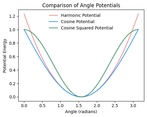
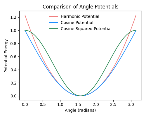
Fig. 2.18 Comparison of harmonic, cosine, and cosine-squared angle potentials, all with an angle constant \(k=1\) and a set angle \(\theta_0\) of \(\pi/2\).

2.4.3. Dihedral Potentials

Torsional or dihedral angles are defined as shown in Fig. 2.19. One needs to define two planes created by three of the four points each.

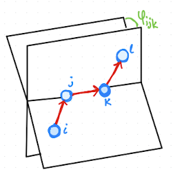
Fig. 2.19 Definition of dihedral or torsional angle.

Angle between two plane (A,B) normals:

• \( \vec{n}_A = \vec{r}_{ij} \times \vec{r}_{jk} \)

• \( \vec{n}_B = \vec{r}_{jk} \times \vec{r}_{kl} \)

Then the angle is

\(\varphi_{ijkl} = \frac{\vec n_A \cdot \vec n_B}{|n_A||n_B|}\)

Similar to the angle, alternative definitions exist, \(\psi = \pi -\varphi\).

To compute dihedral forces on four particles, we need to compute

\[\begin{split} F_i &= -\nabla_i U_\phi(\phi_{ijkl})\\ &= - \frac{\partial U_\phi}{\partial \phi_{ijkl}} \nabla_i \phi_{ijkl} \\ &= - \frac{\partial U_\phi}{\partial \phi_{ijkl} } \frac{\partial \phi_{ijkl}}{\partial \cos(\phi_{ijkl})} \nabla_i \cos\phi_{ijkl} \\ &= -F_\phi \frac{1}{\sin(\phi_{ijkl})} \nabla_i \cos\phi_{ijkl}\quad . \end{split}\]

This results in some involved computations, see Allen & Tildesley¹ for a step by step derivation in Appendix C.

Warning

The same singularities as for the angle forces show up at \(\phi_{ijkl}=0^\circ\) and \(180^\circ\) but one can eliminate them (details in Bondel, Karplus, J. Comput. Chem., 17: 1132-1141, 1996)².

However, \(\phi\) becomes also degenerate if \(\theta_{ijk}\) or \(\theta_{jkl}\) approaches \(0^\circ\) or \(180^\circ\) because the two planes to define the dihedral cannot be defined in these cases. This is important for models with “soft” interactions, where these configurations are possible, e.g. coarse-grained models.

2.4.3.1. Periodic

\[ V_\phi(\phi_{ijkl}) = k_{\phi}(1 + \cos(n \phi - \phi_s)) \quad . \]

Used in the CHARMM force field

2.4.3.2. Ryckaert-Bellemans

\[ V_{\phi}(\phi_{ijkl}) = \sum_{n=0}^5 C_n( \cos(\psi ))^n, \text{ where } \psi = \phi -180^\circ\quad . \]

2.4.3.3. Fourier

\[ V_{F} (\phi_{ijkl})= \frac{1}{2} \sum_{n=1}^4 C_n (1-(-1)^n\cos(n\phi)) \]

Used in the OPLS force field. This can be transformed into the Ryckaert-Bellemans form using trigonometric indentities.

2.4.4. Improper Dihedrals

In addition to the dihedrals defined between four bounded particles in a row, there are also so called improper dihedrals, that can be applied to keep planar groups planar, or prevent flipping into mirror images. These are commonly applied between four points in configurations as sketched in Fig. 2.20.

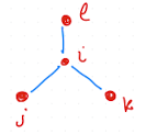
Fig. 2.20 Configuration to which an improper dihedral can be applied to.

2.4.5. References

• Allen & Tildesley, “Simulations of liquids” Appendix C.2 - Calculation of forces and torques ¹

• “Note: Smooth torsional potentials for degenerate dihedral angles” Michael P. Howard, Antonia Statt, Athanassios Z. Panagiotopoulos, J. Chem. Phys. 146, 226101 (2017)⁶

• Blondel, A. and Karplus, M., “New formulation for derivatives of torsion angles and improper torsion angles in molecular mechanics: Elimination of singularities.” J. Comput. Chem., 17: 1132-1141. (1996)²

• Gromacs Documentation on Intramolecular Potentials