4.4. Langevin Dynamics

4.4.1. Implicit-Solvent Models

An implicit-solvent model represents average solvent molecules using the idea of “effective potentials”.

In previous discussions, we defined the forcefield and captured all molecular interactions using a microcanonical ensemble (NVE). However, when switching to the practical canonical ensemble (NVT), the computational cost increases with the thermostat dynamics. Especially for a large system, simulating non-target solvent molecules is neither meaningful nor necessary.

Example: Simulate nanoparticles in a solvent. If we use an explicit solvent model, our system looks like this.

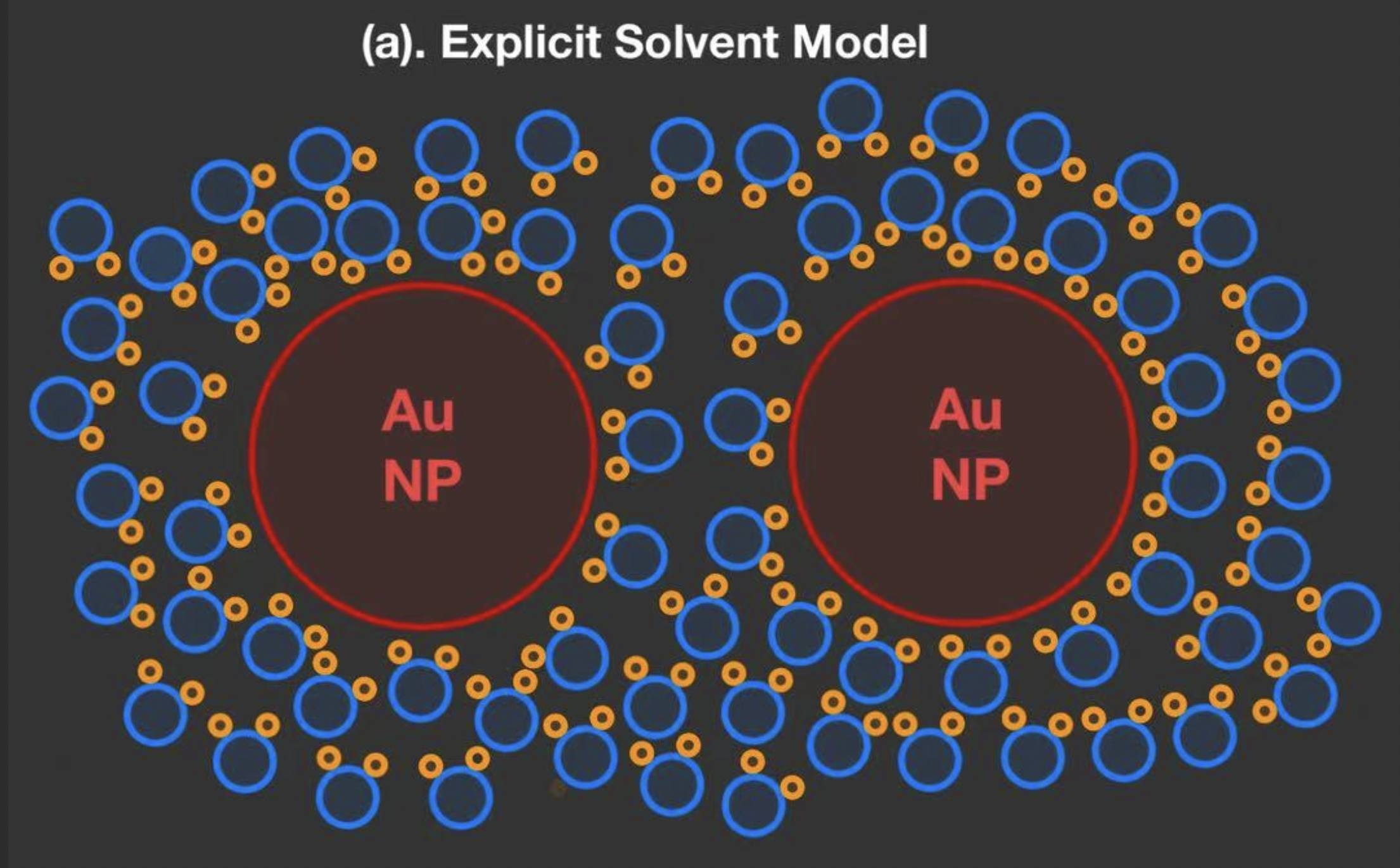
Fig. 4.2 Schematic of the visualization for a modeling of Au nanoparticles in water by explicit solvent model.

• While we need to define the detailed atomic arrangements in Au Nanoparticles, we also need to model the structure of water molecules.

• The slowest part of an MD simulation is calculating the distances and forces of all particles. In this case, we need to calculate these parameters at each timestep for each NPs and water molecule.

• Note that in an actual simulation, there will be more than the number of water molecules drawn in the schematic (approximately \(10^6\) depending on the system).

An implicit solvent model treats solvent molecules as a “bath”, which transfers the molecular interactions to averaged, continuum effects with the frictional drag and stochastic force.

• Frictional drag: Energy dissipation into the surrounding implicit solvent.

• Stochastic force: A random kick from the solvent that simulates the collisions of solvent molecules and keeps the system at constant temperature.

Example: Simulate nanoparticles in a solvent.

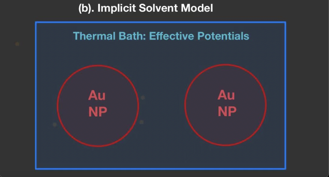
Fig. 4.3 Schematic of the visualization for a modeling of Au nanoparticles in water by implicit solvent model.

• The system only contains the Au nanoparticles. But the frictional drag and stochastic force are added in the force term.

• The thermal bath can exchange heat with Au nanoparticles. Essentially, the Au nanoparticles can “feel” the solvent molecules.

4.4.2. Langevin Dynamics

The bridge connecting the explicit molecular interactions with the implicit forces is called the Langevin dynamics, as the “thermal bath” above.

4.4.3. Fluctuation-dissipation theorem

“When there is a process that dissipates energy, turning into heat, then there is a reverse process related to thermal fluctuations.”

Example:

• The Au nanoparticles experience the drag (fluid resistance) from solvent molecules. Then, the drag dissipates kinetic energy, turning it into heat. (Kinetic energy to heat)

• Conversely, the Au nanoparticles move around with a change in velocity when molecules collide based on the Brownian motion. (Heat to kinetic energy)

Conceptually, Langevin dynamics can be split into 2 parts:

• Thermodynamics: Random thermal noise and dissipative processes (friction, damping) are not independent. Balancing the energy distribution ensures constant T.

• Dynamics: Drag force from viscous friction is balanced with thermal kicks in damping. Allow the simulation of Brownian motion.

4.4.4. Langevin Equation

Mathematically, the Langevin dynamics can be defined in the same logic.

• Balancing the stochastic thermal noise with the viscous drag modify the momentum of the system.

Langevin Equation $\( mdv = \big(F(r(t)) - \gamma v\big)\,dt + \sigma\,dW_t \)$

\(F(r(t))\): Conservative forces originate from the system, such as intermolecular potentials.

\(\gamma\): Friction coefficient, $$ represents the viscous drag force.

The friction coefficient \(\gamma\) can be approximated by \(\gamma = 6 \pi \eta a\), where \(\eta\) is the the dynamic viscosity of the medium and \(a\) is the radius of particle.

\(\sigma\): Strength of fluctuations, $$ represents the stochastic thermal force.

\(W_t\) is the Wiener process, which is the cumulative Brownian random motion. \(d W_t\) is the Wiener increment as the infinitesimal step of the Brownian motion with \(\langle dW_t \rangle = 0, \,\,\langle dW_t^2 \rangle = dt\).

• To show the conservation of T for the canonical ensemble can be realized by linking thermal fluctuation and viscous drag, Itô’s lemma is used to capture the stochastic relationship in a 1-D example.

\[ mdv = \big(F(r(t)) - \gamma v\big)\,dt + \sigma\,dW_t \,\, \rightarrow \,\, dv = A(v,t) \,dt + B(v, t) \, dW_t \]

Since \(F(r(t))\) is the deterministic Newton’s Second Law, it will not be included in the discussion of kinetic energy dissipation and injection.

Similar to the transformation of thermodynamic variables, for a given function \(f = f(v, t)\), it can be expressed with the above equation.

\[ df = \frac{\partial f}{\partial t}\, dt + \frac{\partial f}{\partial v}\, dv \,\, \rightarrow \,\, df = f_t \, dt + f_v \, dv \]

As \(\langle dW_t \rangle = 0, \,\, \langle dW_t^2 \rangle = dt\), substituting \(dv\) with \(A(v,t) \,dt + B(v, t) \, dW_t\). Since \(d W_t\) is a stochastic term, it is expanded and considered up to 2nd order.

\[ df = f_t \, dt + f_v \, dv + \frac{1}{2} f_{vv} \, (dv)^2 \]

\[ df = f_t \, dt + f_v \, (A(v,t) \,dt + B(v, t) \, dW_t) + f_{vv} \, (A(v,t) \,dt + B(v, t) \, dW_t)^2 \]

Using Itô’s lemma, \((dt)^2 = 0,\, dt dW_t = 0, \, (d W_t)^2 = dt\).

\[ df = (f_t + A f_v + \frac{1}{2} B^2 f_{vv}) \ dt + B f_v \, dW_t \]

The first part \((f_t + A f_v + \frac{1}{2} B^2 f_{vv}) \ dt\) describes the drift of the function \(f(v, t)\), and the second part \(B f_v \, dW_t\) describes the random fluctuations. Taking the average using Itô’s lemma, we identify the relationship with the stochastic term average to 0.

\[ \frac{d}{dt} \langle f \rangle = \langle A f_v + \frac{1}{2} B^2 f_{vv} \rangle \]

To investigate thermal equilibrium, \(f(v, t)\) can be set as the kinetic energy and say \(f \propto v^2\). With \(A(v,t) = - \frac{\gamma}{m}v, \, \, B(v,t) = \frac{\sigma}{m}\).

\[ \frac{d}{dt} \langle v^2 \rangle = - \frac{2 \gamma}{m} \langle v^2 \rangle + \frac{\sigma^2}{m^2} \]

At constant temperature, the Maxwell-Boltzmann distribution suggests that the velocity variance is no longer changed.

\[ 0 = - \frac{2 \gamma}{m} \langle v^2 \rangle + \frac{\sigma^2}{m^2} \,\, \rightarrow \,\, \langle v^2 \rangle = \frac{\sigma^2}{2m\gamma} \]

From thermodynamics, the average kinetic energy per degree of freedom is:

\[ \frac{1}{2} m \langle v^2 \rangle = \frac{1}{2} k_B T \,\, \rightarrow \,\, \frac{1}{2} m (\frac{\sigma^2}{2m\gamma}) = \frac{1}{2} k_B T \]

Fluctuation-dissipation relation

\[ \sigma^2 = 2\gamma k_B T \]

Therefore, the strength of fluctuations \(\sigma\) is dependent on the friction coefficient \(\gamma\) under this stochastic process. Intuitively, large friction between molecules requires larger thermal fluctuations to maintain the same T.

This coupling verifies that the Langevin dynamics is a valid thermostat, which maintains the correct thermal distribution.

To integrate the Langevin dynamics, one way is to add the viscous drag and thermal fluctuation directly to the Velocity Verlet algorithm.

Example: Velocity Verlet

1. Half-step velocity update:

\[ v\!\left(t+\frac{\Delta t}{2}\right) = v(t) + \frac{\Delta t}{2m} F(t) \,\, \rightarrow \,\, v\!\left(t+\frac{\Delta t}{2}\right) = v(t) + \frac{\Delta t}{2m} F(t) - \frac{\gamma \Delta t}{2}v(t) + \frac{\sigma}{2m}G_1\sqrt{\Delta t} \]

2. Full-step position update, note that the velocity includes drag and noise:

\[ x(t+\Delta t) = x(t) + \Delta t \, v\!\left(t+\frac{\Delta t}{2}\right) \]

3. Half-step velocity update:

\[\begin{split} \begin{aligned} v(t+\Delta t) &= v\!\left(t+\frac{\Delta t}{2}\right) + \frac{\Delta t}{2m} F(t+\Delta t) \\ &\rightarrow v(t+\Delta t) = v\!\left(t+\frac{\Delta t}{2}\right) + \frac{\Delta t}{2m} F(t+\Delta t) - \frac{\gamma \Delta t}{2}v\!\left(t+\frac{\Delta t}{2}\right) + \frac{\sigma}{2m}G_2\sqrt{\Delta t} \end{aligned} \end{split}\]

Note that \(G_1 G_2\) are random standardized Gaussian variables, they represent the thermal noise and are independent of each other so \(\langle G_1 G_2\rangle = 0\).

However, to retain symplectic properties, sophisticated schemes are highly recommended. A good reference for sophisticated algorithms that implement Langevin dynamics is “[Robust and efficient configurational molecular sampling via Langevin dynamics, Leimkuhler; Matthews, J. Chem. Phys. 138, 174102 (2013)]”.

One popular algorithm is “BAOAB”, which means “B (force) \(\rightarrow\) A (drift) \(\rightarrow\) O (thermostat) \(\rightarrow\) A (drift) \(\rightarrow\) B (force)”.

Example: BAOAB Scheme

Step 1: Half step momentum update.

\[ \textbf{B:}\quad \mathbf{p}_{\frac{1}{2}} (\frac{\Delta t}{2}) \;=\; \mathbf{p}(0)\;+\;\frac{\Delta t}{2}\,\mathbf{F}\!\big(\mathbf{r}(0)\big) \]

Step 2: Half step position update.

\[ \textbf{A:}\quad \mathbf{r}_{\frac{1}{2}} (\frac{\Delta t}{2}) \;=\; \mathbf{r}(0)\;+\;\frac{\Delta t}{2m}\,\mathbf{p}_{\frac{1}{2}} (\frac{\Delta t}{2}) \]

Step 3: Ornstein - Uhlenbeck thermostat update for force.

\[ \textbf{O:}\quad \mathbf{p}'_{\frac{1}{2}} (\frac{\Delta t}{2}) \;=\; e^{-\frac{\gamma\,\Delta t}{m}}\mathbf{p}_{\frac{1}{2}} (\frac{\Delta t}{2}) \;+\;\sqrt{\,m k_B T\,\Big(1 - e^{-\frac{2\gamma\,\Delta t}{m}}\Big)}\,\mathbf{G}, \qquad \mathbf{G}\sim\mathcal{N}(\mathbf{0},\mathbf{I}) \]

Step 4: Half step position update.

\[ \textbf{A:}\quad \mathbf{r}(\Delta t) \;=\; \mathbf{r}_{\frac{1}{2}} (\frac{\Delta t}{2})\;+\;\frac{\Delta t}{2m}\,\mathbf{p}'_{\frac{1}{2}} (\frac{\Delta t}{2}) \]

Step 5: Half step momentum update.

\[ \textbf{B:}\quad \mathbf{p}(\Delta t) \;=\; \mathbf{p}'_{\frac{1}{2}} (\frac{\Delta t}{2})\;+\;\frac{\Delta t}{2}\,\mathbf{F}\!\big(\mathbf{r}(\Delta t)\big) \]

This structure symmetrically splits the deterministic and stochastic updates, which is time-reversible.

The BAOAB algorithm is superior in position space. The steady-state positional distribution is exact up to \(O((\Delta t)^4)\). This is important for the NVT ensemble, which preserves the exact Maxwell-Boltzmann distribution for positions.

The A-step and B-step are the same as the half-step position and velocity updates in the Velocity Verlet algorithm. Therefore, the deterministic part of the BAOAB algorithm is symplectic. However, the O-step breaks Liouville’s theorem with the friction.

\[\begin{split} \begin{cases} \mathbf{r}' = \mathbf{r}, \\ \mathbf{p}' = e^{-\frac{\gamma \Delta t}{m}} \mathbf{p} + \sqrt{m k_B T \left( 1 - e^{-2 \frac{\gamma \Delta t}{m}} \right)}\, \mathbf{G} \end{cases} \end{split}\]

\[ \frac{\partial \mathbf{r}'}{\partial \mathbf{r}} = \mathbf{I}, \qquad \frac{\partial \mathbf{r}'}{\partial \mathbf{p}} = 0, \qquad \frac{\partial \mathbf{p}'}{\partial \mathbf{r}} = 0, \qquad \frac{\partial \mathbf{p}'}{\partial \mathbf{p}} = c\,\mathbf{I} \]

\[\begin{split} J_O = \begin{pmatrix} \mathbf{I} & 0 \\ 0 & e^{-\frac{\gamma \Delta t}{m}}\,\mathbf{I} \end{pmatrix} \;\Rightarrow\; \det(J_O) = \det(\mathbf{I}) \cdot \det\!\left(e^{-\frac{\gamma \Delta t}{m}}\,\mathbf{I}\right) = e^{-3\,\frac{\gamma \Delta t}{m}} \leq 1 \end{split}\]

As the frictional coefficient \(\gamma > 0\), the frictional force leads to the contraction in phase space volume. Energy is lost to the heat bath, but the stochastic random noise reinjects the energy and balances the dissipation on average. So the average energy stays constant at equilibrium and yields the correct Boltzmann distribution at steady state.

4.4.5. Brownian Dynamics

As we showed before \(\sigma^2 = 2\gamma k_B T\), the friction coefficient \(\gamma\) is highly dependent on the strength of fluctuation \(\sigma\).

If \(\gamma \rightarrow 0\), then from the equation \(\sigma \rightarrow 0\), the equation left is the pure deterministic Newton’s second law \(m \frac{d v}{dt} = F (\mathbf{r} (t))\).

For the Langevin equation \(mdv = \big(F(\mathbf{r}(t)) - \gamma v\big)\,dt + \sigma\,dW_t\), the equation is very similar to the damping equation \(m \ddot{x} + \gamma \dot{x} + kx = 0\) with the damping ratio \(\zeta = \frac{\gamma}{2 \sqrt{km}}\).

If the damping ratio \(\zeta\) is very large, which means the system is friction-dominated, then \(\gamma\) is very large. The system does not exhibit any oscillation behaviors, and the relaxation process is very slow. Conceptually, damping is the resistance to motion, which is the frictional drag that constantly pulls the system back to rest.

At high \(\gamma\), the system velocity would not pick up, thus the friction overcomes the inertia term \(m \frac{dv}{dt}\). Then, the system would only follow the random thermal kicks or other external forces in the environment. An analogy for this is “a pendulum in thick honey”, which would never oscillate but respond to the thermal kicks from the honey molecules if we try to heat the honey.

In the above scenario, at the overdamped limit, for a 1-D system:

\[ 0 = F(r(t)) - \gamma v + dW_t \]

Solve for \(v\) then the equation changes to:

\[ v(t) = \frac{F(r(t))}{\gamma} + \frac{\sigma}{\gamma} d W_t \]

Then, substitute \(dx = v dt\) , the system reduces to position-only dynamics as the Brownian equation.

\[ dx = \frac{F(r(t))}{\gamma} dt + \frac{\sigma}{\gamma} dW_t \]

By the fluctuation-dissipation theorem \(\sigma^2 = 2\gamma k_B T\), the thermal fluctuation strength can be substituted with \(\gamma\).

\[ dx = \frac{F(r(t))}{\gamma} dt + \sqrt{\frac{2 k_B T}{\gamma}} dW_t \]

The Stokes-Einstein equation defines the diffusion coefficient \(D\) as \(D = \frac{k_B T}{\gamma}\).

\[ dx = \frac{F(r(t))}{\gamma} dt + \sqrt{2D} dW_t \]

Different components of the random displacement are statistically independent, therefore, the correlation of the process can be described by the delta function:

\[ \langle G_i\,G_j \rangle = 2D\,\Delta t\,\delta_{ij} \]

The Brownian equation describes the motion of a particle in highly viscous environments. At each infinitesimal timestep, the particle moves in the direction of force with a velocity of \(\frac{F(r(t))}{\gamma}\) and diffuses due to the random thermal kick by the surrounding fluid.

A good example of the Brownian motion is the Perrin experiment, where the experiment used a microscope to observe the three tracings of the motion of colloidal particles of radius \(0.53 \mu m\).

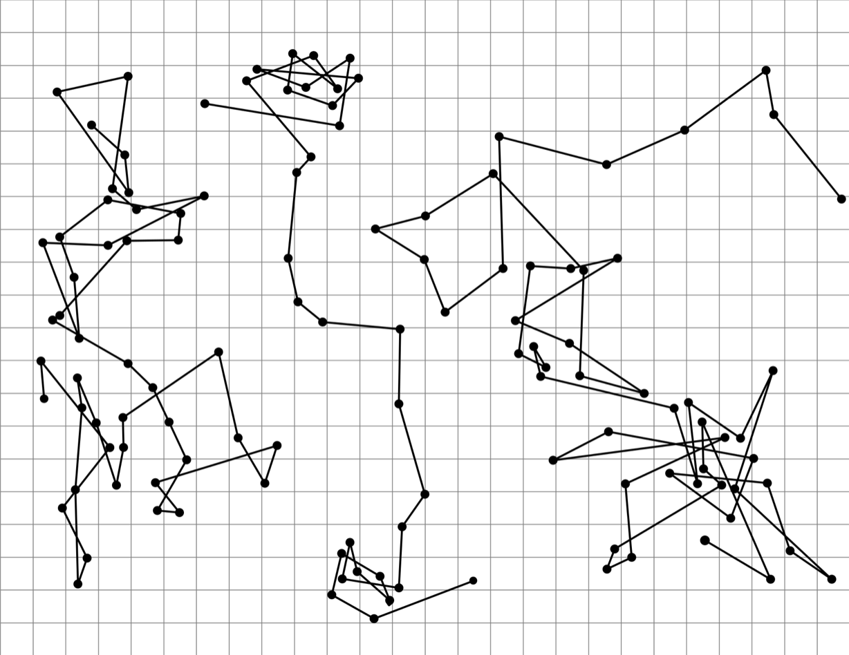
Fig. 4.4 The Colloidal motions under microscope in Perrin experiment.

Recall from the previous discussion, the diffusion coefficient can also be measured by the mean-square displacement \(\langle \Delta r(t)^2 \rangle\).

\[ \langle \Delta r(t)^2 \rangle = 2 d D t \,\, \text{(d: dimension)} \]

For the Brownian equation, suppose \(F = 0\), then the equation can be integrated, and take average can be taken to compare with the mean square displacement.

\[ dx = \sqrt{2D} dW_t \]

\[ x(t) - x(0) = \int_0^t \sqrt{2D} \, dW_t = \sqrt{2D} (W_t - W_0) \]

The mean of the motion is 0, as the expectation value of the Wiener process is 0.

\[ \mathrm{E}[W_t] = 0 \rightarrow \mathrm{E}[\sqrt{2D} (W_t - W_0)] = 0 \]

The variance can be calculated through Itô’s isometry for any square-integrable process:

\[ \mathrm{E}\!\left[\left(\int_0^t g_t\, dW_t \right)^2\right] = \mathrm{E}\!\left[\int_0^t g_t^2\, dt \right] \]

\[ \mathrm{Var} [x(t) - x(0)] = \mathrm{E}\!\left[ \int_0^t \sqrt{2D} \, dW_t\right] = \mathrm{E}\!\left[ \int_0^t 2D \, dt\right] = 2Dt \]

Therefore, the mean square can be calculated as:

\[ \mathrm{E}[X^2] = \mathrm{E}[X]^2 + \mathrm{Var}[X] = 2Dt \rightarrow \text{MSD} = 2dDt \,\, \text{(d: dimension)} \]

The Brownian motion equation is thus verified by the Perrin experiment and the Stokes-Einstein equation, confirming the fluctuation–dissipation picture that underlies Langevin dynamics.

Discrete update rule for the Brownian Dynamics

To implement in computational work, integrate the Brownian motion with a timestep \(\Delta t\):

\[ \mathrm{d}\mathbf{x} = \frac{\mathbf{F}(\mathbf{r}(t))}{\gamma}\,\mathrm{d}t + \sqrt{\frac{2 k_B T}{\gamma}}\,\mathrm{d}\mathbf{W}_t \rightarrow \mathbf{x}(\Delta t)-\mathbf{x}(0) = \int_{0}^{\Delta t}\frac{\mathbf{F}(\mathbf{r}(t))}{\gamma}\,\mathrm{d}t + \int_{0}^{\Delta t}\sqrt{\frac{2 k_B T}{\gamma}}\,\mathrm{d}\mathbf{W}_t \]

For a small timestep \(\Delta t\), we can approximate the results by Euler’s method:

\[ \mathbf{x}(\Delta t) \approx \mathbf{x}(0) + \frac{\mathbf{F}(\mathbf{x}(0))}{\gamma}\,\Delta t + \sqrt{\frac{2 k_B T}{\gamma}}\bigl(\mathbf{W}_{\Delta t}-\mathbf{W}_0\bigr) \]

The change in the Wiener process can be assumed as Gaussian with a variance of \(\Delta t\).

\[ \mathbf{W}_{\Delta t}-\mathbf{W}_0 = \sqrt{\Delta t}\,\mathbf{G}, \qquad \mathbf{G}\sim\mathcal{N}(\mathbf{0},\mathbf{I}) \]

Therefore, the update rule can be expressed as:

\[ \mathbf{x}(\Delta t) = \mathbf{x}(0) + \frac{\mathbf{F}(\mathbf{x}(0))}{\gamma}\,\Delta t + \sqrt{\frac{2 k_B T\,\Delta t}{\gamma}}\,\mathbf{G} \qquad \mathbf{G}\sim\mathcal{N}(\mathbf{0},\mathbf{I}) \]

4.4.6. Hydrodynamic Interactions

When particles are under Brownian motion through a viscous solvent, they disturb the surrounding fluid and create a Stokes flow. However, the flow itself is not localized, but exerts a drag effect on nearby particles. Therefore, the motions of particles alter the velocity field that can be “felt” by all others. The phenomenon is called the hydrodynamic effect.

The displacement or force on one particle propagates through the viscous fluid, inducing correlated motion in the rest of the system.

A good reference that discussed hydrodynamic interaction is [Brownian dynamics with hydrodynamic interactions, Ermak; McCammon, J. Chem. Phys. 69, 1352 (1978); doi: 10.1063/1.436761].

For the Brownian particles, a generalized overdamped Langevin equation with the effect of the velocity field can be described by adjusting the velocity of each particle with a mobility tensor \(\mathbf{M}\).

\[ \mathbf{v}_i = \sum_j \mathbf{M}_{ij} \mathbf{F}_j \]

The full mobility tensor matrix is defined as a $$ symmetric matrix:

\[\begin{split} \begin{equation} \mathbf{M} = \begin{pmatrix} \mathbf{M}_{11} & \mathbf{M}_{12} & \cdots & \mathbf{M}_{1N} \\ \mathbf{M}_{21} & \mathbf{M}_{22} & \cdots & \mathbf{M}_{2N} \\ \vdots & \vdots & \ddots & \vdots \\ \mathbf{M}_{N1} & \mathbf{M}_{N2} & \cdots & \mathbf{M}_{NN} \end{pmatrix} \end{equation} \end{split}\]

where each block defines how a force on particle \(j\) produces a velocity on particle \(i\).

To construct the mobility matrix, each term can be found by the following categories:

(a). Self-mobility (\(i = j\))

\[ \begin{equation} \mathbf{M}_{ii} = \frac{1}{6\pi\eta a}\,\mathbf{I} \end{equation} \]

where \(a\) is the solvent radius and \(\eta\) is the solvent viscosity.

(b). Long-range coupling - Oseen tensor (\(i \neq j\))

\[ \begin{equation} \mathbf{M}_{ij} = \frac{1}{8\pi\eta r_{ij}} \big( \mathbf{I} + \hat{\mathbf{r}}_{ij}\hat{\mathbf{r}}_{ij} \big), \quad i \neq j \end{equation} \]

where \(\mathbf{r}_{ij} = \mathbf{r}_i - \mathbf{r}_j\) is the distance between 2 particles.

A long-range tensor can be found with Ewald sums through [Fiore et al., J. Chem. Phys., 146, 12416 (2019)], which decomposes \(\mathbf{M}_{ij}\) into a short-range “real-space” part and a long-range “wave-space” part using the Fourier transform. Then, the short range can be evaluated through the neighbor list, while the long range can be evaluated through the Fourier transform.

©. Rotne–Prager tensor (finite-size correction \(r_{ij} \geq 2a\))

\[ \begin{equation} \mathbf{M}_{ij} = \frac{1}{8\pi\eta r_{ij}} \left[ \left( 1 + \frac{2a^2}{3r_{ij}^2} \right)\mathbf{I} + \left( 1 - \frac{2a^2}{r_{ij}^2} \right)\hat{\mathbf{r}}_{ij}\hat{\mathbf{r}}_{ij} \right] \end{equation} \]

This correction ensures that the final mobility tensor matrix is symmetric and positive definite, where \(\mathbf{M}_{ij} = \mathbf{M}_{ji}\), thereby providing stable stochastic integration.

Physically, \mathbf{M}_{ij} is the hydrodynamic response tensor for interactions between particle \(i\) and particle \(j\), which is the fluid velocity at \(i\) induced by a unit force on \(j\).

For the particle \(i\), a generalized overdamped Langevin equation with the solvent-mediated effect is described as:

\[ \begin{equation} \dot{\mathbf{x}}_i = \sum_j \mathbf{M}_{ij}(\mathbf{r})\,\mathbf{F}_j + \boldsymbol{\xi}_i(t) \end{equation} \]

\(\dot{\mathbf{x}}_i\): the velocity of particle \(i\).

\(\mathbf{F}_j\): the total deterministic force exerted on particle \(j\).

\(\boldsymbol{\xi}_i (t)\): random noise term of particle \(i\).

For a given particle \(i\) and particle \(j\), the fluctuation-dissipation theorem can be satisfied by the correlated fluctuations:

\[ \begin{equation} \left\langle \boldsymbol{\xi}_i(t)\, \boldsymbol{\xi}_j(t')^{\mathrm{T}} \right\rangle = 2 k_B T\, \mathbf{M}_{ij}(\mathbf{r})\, \delta(t - t') \end{equation} \]

Integrate over a small timestep \(\Delta t\), the update rule can be expressed as:

\[ \begin{equation} \mathbf{x}(\Delta t) = \mathbf{x}(0) + \big( \mathbf{M}\cdot\mathbf{f} + k_B T\, \nabla\cdot\mathbf{M} \big)\Delta t + \mathbf{B} \end{equation} \]

\[ \begin{equation} \langle \mathbf{B}\mathbf{B}^{\mathrm{T}} \rangle = 2 k_B T\, \mathbf{M}\, \Delta t \end{equation} \]

In theory, the random thermal fluctuation term \(\mathbf{B}\) can be calculated with the mobility matrix \(\mathbf{M}\).

\[ \begin{equation} \mathbf{B} = \sqrt{2k_B T\, \Delta t}\, \mathbf{M}^{1/2}\, \mathbf{G} \end{equation} \qquad \mathbf{G}\sim\mathcal{N}(\mathbf{0},\mathbf{I}) \]

While \(\mathbf{M}^{1/2}\) can be solved through the Eigen-decomposition method (not efficient), another way to solve this is to perform free drawing from the known covariance of the mobility operator. Based on [Fiore et al., J. Chem. Phys., 146, 12416 (2019)], a known Brownian noise can be drawn as:

\[ \Delta\mathbf{x}_B = \sqrt{2k_B T\,\Delta t}\; \big( \mathbf{M}^{(r)\,1/2}\,\mathbf{G}_r + \mathbf{M}^{(w)\,1/2}\,\mathbf{G}_w \big) \]

Here, both \(\mathbf{M}^{(r)\,1/2}\) (computed by local neighbor list) and \(\mathbf{M}^{(w)\,1/2}\) (computed by the Fourier transform) are known positive definite and symmetric matrices, then by drawing independent Gaussian vectors through \(\mathbf{G}_r, \mathbf{G}_w \sim\mathcal{N}(\mathbf{0},\mathbf{I})\) can still generate Brownian noise without solving a complicated linear system.

Therefore, for selected particles \(i\) and \(j\), their motions are correlated based on the mobility matrix:

\[ \begin{equation} \left\langle \Delta\mathbf{r}_i\, \Delta\mathbf{r}_j^{\mathrm{T}} \right\rangle = 2 k_B T\, \mathbf{M}_{ij}\, \Delta t \end{equation} \]

As in the previous discussion, the Brownian motion describes the diffusion process in the stochastic term. It is noticeable that the above discussion can be connected to non-equilibrium thermodynamics.

\[ \text{Fluxes} = \text{(transport coefficients)} \cdot \text{(driving forces)} \]

• In Brownian dynamics, a force on one particle induces motion of another via solvent flow.

• In kinetics, a gradient in one variable (say temperature) can drive another flux (say mass or charge).

Onsager’s formalism, derived from nonequilibrium thermodynamics, provides a similar setup here:

\[ \mathbf{v}_i = \sum_j \mathbf{M}_{ij} \mathbf{F}_j \Leftrightarrow \mathbf{J}_i = -\sum_j \mathbf{L}_{ij} \nabla \mathbf{\mu}_j \]

In addition, the Onsager’s coefficients also have the property of being symmetric, positive definite, with \(\mathbf{L}_{ij} = \mathbf{L}_{ji}\) here, same as the mobility tensor \(\mathbf{M}_{ij} = \mathbf{M}_{ji}\).

• If particle \(j\) induces motion in particle \(i\) through the solvent, then particle \(i\) would induce the same motion in \(j\) if their roles were reversed.

• Every dissipative process in a near-equilibrium system has a symmetric, fluctuation-linked transport matrix that couples fluxes and forces.

• The Hydrodynamics interactions, in essence, quantify how equilibrium fluctuations and dissipation are intertwined through microscopic reversibility.

4.4.7. Langevin Thermostat: Conclusion

By making γ small, the Langevin Dynamics can be used as a thermostat without significantly perturbing the system.

• A value γ ≈ 0.1 m/Å is usually considered “weak” coupling and good for thermostating.

• Beware: Langevin thermostat does not conserve momentum (forces do not sum to zero). Hence, there are no zero degrees of freedom.

• Hydrodynamics of an explicit solvent with Langevin thermostat may also get screened due to lack of momentum conservation.

Langevin thermostat is an intermediate approach compared to Nosé–Hoover thermostat (deterministic and momentum conserved) and Andersen thermostat (stochastic reassignment but disrupts real dynamics). Hence, Langevin dynamics are often preferred for biomolecular, nanoparticle, and diffusive materials simulations, especially when realistic sampling of phase space is more critical than exact momentum conservation.

4.4.8. References

• Allen & Tildesley, “Simulations of liquids” Appendix B - Reduced Units ²

• Seifert, U. (2025). Stochastic Thermodynamics. Cambridge University Press. ³³

• Gardiner, C. W. (2009). Stochastic Methods: A Handbook for the Natural and Social Sciences. Springer. ¹⁰

• Ermak, D. L., & McCammon, J. A. (1978). Brownian dynamics with hydrodynamic interactions. J. Chem. Phys., 69(4), 1352–1360. ⁷

• Kubo, R. (1966). The fluctuation–dissipation theorem. Rep. Prog. Phys., 29(1), 255–284. ¹⁸

• Risken, H. (1996). The Fokker–Planck Equation: Methods of Solution and Applications. Springer. ³¹

• van Kampen, N. G. (2007). Stochastic Processes in Physics and Chemistry. North-Holland. ⁴⁴

• Leimkuhler, B., & Matthews, C. (2013). Robust and efficient configurational molecular sampling via Langevin dynamics. J. Chem. Phys., 138(17), 174102. ²⁰

• R. W. Balluffi, S. A. Allen, W. C. Carter (2005), Kinetics of materials, John Wiley & Sons, Inc. ³