4.3. Thermostats

4.3.1. Generate canonical ensemble in MD

Before, we covered how the Velocity Verlet algorithm can be implemented to perform a microcanonical ensemble (NVE). The Velocity Verlet algorithm provides an efficient, time-reversible, and symplectic approach for simulating materials with a constant number of particles (N), constant system volume (V), and a constant total energy (E).

Experimentalists may not be happy about this, as the system volume and the total energy are very hard to control in real experiments. Practically, it is much easier to control the pressure (P) and temperature (T) experimentally. Ideally, an isothermal-isobaric NPT ensemble is the best to simulate the particles, just like doing an experiment. With the NPT ensemble, the phase of the system is unique based on the phase diagram. Then, phenomena such as phase transitions can be directly captured through precise temperature and pressure controls.

In this section, we will first focus on changing the constant energy (E) to constant temperature (T) with an implementation called thermostat. Adding a thermostat to the original MD simulation setup changes our system from a microcanonical ensemble (NVE) to a canonical ensemble (NVT). With a thermostat, the system is allowed to exchange energy with a heat bath, which is just like a large reservoir for an experimentalist, so the kinetic energy of atoms can be regulated. It also mimics thermal fluctuations of atoms in a real physical system. A thermostat is exactly like the one you have in your home, where the thermostat drives the simulated system to the target temperature, like an “air conditioner.”

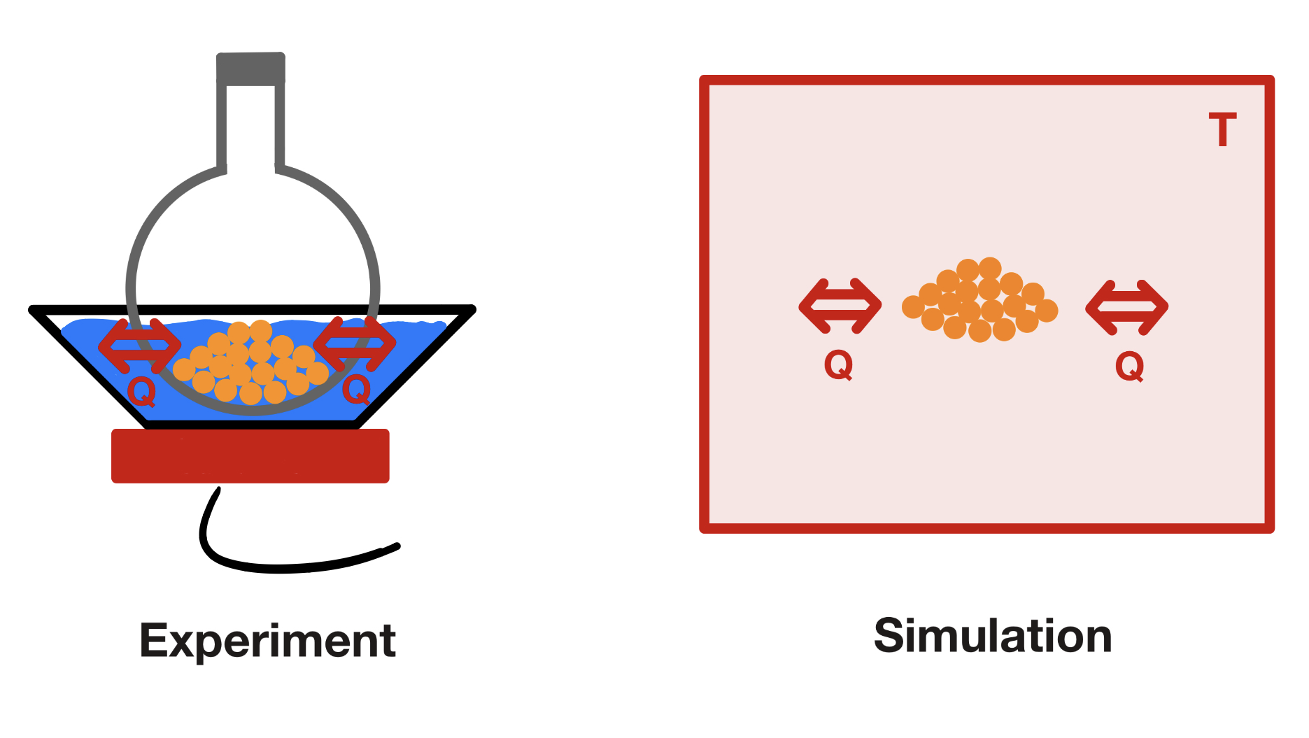
Fig. 4.1 Schematic of the visualization for a heat bath for simulation.

Ultimately, thermostats bridge the gap between theoretical ensembles and realistic simulations. They enable MD systems to reproduce experimental thermodynamic conditions while maintaining stable numerical integration, making them indispensable tools in computational materials science and statistical mechanics.

As a reminder, while it is convenient to use open-source packages like LAMMPS, HOOMD-blue, and GROMACS, it is very important to check how the thermostats are defined and implemented so your simulations are physically reliable and reproducible.

4.3.2. Microscopic and macroscopic connectivity of the thermostat

In an atomic view, the temperature is described by the average kinetic energy per atom. Recall that the Maxwell-Boltzmann distribution describes the probability that a particle in thermal equilibrium has a velocity \(\mathbf{v}\) and magnitude \(v\).

\[ f(\mathbf{v}) = (\frac{m}{2 \pi k_B T})^{\frac{3}{2}} \,\mathrm{exp}\,(-\frac{m (v_x^2 + v_y^2 + v_z^2)}{2 k_B T}) \quad d^3v = dv_x dv_y dv_z \]

For directions \(\alpha = (x,y,z)\), it can be factorized into three independent 1-D Gaussians:

\[ f(\mathbf{v}) = f_x (v_x) \, f_y (v_y) \, f_z (v_z) \quad \leftarrow \quad f_{\alpha} (v_\alpha) = (\frac{m}{2 \pi k_B T})^{\frac{1}{2}} \,\mathrm{exp}\,(-\frac{m v_\alpha^2}{2 k_B T}) \]

To find the average kinetic energy per atom, we need to find the mean square velocity, which can be done with the Gaussian integral.

\[ I(a)=\int_{-\infty}^{\infty}e^{-a x^2}dx=\sqrt{\frac{\pi}{a}} \Rightarrow \int_{-\infty}^{\infty} x^{2} e^{-a x^{2}} \, dx = -\frac{d}{da}\!\int_{-\infty}^{\infty} e^{-a x^{2}} dx = -\frac{d}{da}\!\left(\sqrt{\frac{\pi}{a}}\right) = \frac{\sqrt{\pi}}{2\,a^{3/2}} \]

\[\begin{split} \begin{aligned} \langle v_\alpha^2 \rangle &= \int_{-\infty}^{\infty} v_\alpha^2 f_\alpha(v_\alpha)\, dv_\alpha \\ &= \left( \frac{m}{2\pi k_B T} \right)^{1/2} \int_{-\infty}^{\infty} v_\alpha^2 e^{-a v_\alpha^2} \, dv_\alpha \\ &= \left( \frac{m}{2\pi k_B T} \right)^{1/2} \frac{\sqrt{\pi}}{2 a^{3/2}} \\ &= \left( \frac{m}{2\pi k_B T} \right)^{1/2} \frac{\sqrt{\pi}}{2} \left( \frac{2k_B T}{m} \right)^{3/2} \\ &= \frac{k_B T}{m}, \quad (\alpha = x, y, z) \end{aligned} \end{split}\]

\[ \langle v^2 \rangle = \langle v_x^2 + v_y^2 + v_z^2 \rangle = 3 \frac{k_B T}{m} \]

\[ \langle \mathrm{KE} \rangle = N \cdot \frac{1}{2} m \langle v^2 \rangle = \frac{3}{2} N k_B T \]

\[ T = \frac{2}{3 N k_B} \sum_{i = 1}^N \frac{1}{2} m_i v_i^2 \]

Therefore, microscopic motions are closely linked to the macroscopic temperature. The insight for choosing a good thermostat is that it must regulate the correct kinetic energy or conserved momentum.

In addition, the thermostat should not affect the phase-space structure. Similarly, we want to maintain the advantage of Velocity Verlet, where the time-reversible and symplectic integration properties ensure energy conservation in the long run.

4.3.3. Types of thermostats

The type of thermostat is determined by how the thermostat contributes to the kinetic energy ensemble controls.

Stochastic Thermostat: A stochastic process is a fancy way to say “random process”. So the stochastic thermostat means random fluctuations are created from the heat bath. Then, the momenta of the atoms are stochastically updated according to the Maxwell-Boltzmann distribution.

Implementing a stochastic thermostat is usually stable. However, it is noticeable that random number generation would increase the computational cost. In addition, the strength of stochastic fluctuations needs to be carefully controlled, or the random thermal forces would disrupt the conserved momentum and alter the system dynamics.

Deterministic Thermostat: The deterministic thermostats modify the system’s equations of motion by introducing additional scaling variables (frictional drag) that adjust particles’ velocities and ensure that the system evolves toward the target temperature.

A deterministic thermostat is usually accurate when obtaining physically realistic dynamics, as the coupling has no randomness. However, it is often hard to implement the deterministic thermostat correctly to simulate under the canonical ensemble (NVT). One crucial factor is the parameter tuning:

• If the coupling of the frictional drag is too weak, the system may not reach the equilibrium temperature efficiently.

• If the scaling is too large, the mechanical behaviors of the atoms would be completely controlled by the frictional forces, which can lead to non-physical oscillations in temperature.

Langevin Thermostat: A Langevin thermostat introduces both the stochastic thermal fluctuations and the deterministic frictional drag to each particle. The Langevin dynamics controls the system temperatures with a balance between energy dissipation and thermal fluctuation called the fluctuation-dissipation theorem.

It is noticeable that the deterministic friction in the Langevin thermostat is dependent on the stochastic thermal fluctuation strength. The Langevin dynamics is actually adding an “implicit solvent”, where the coupling strength indicates how strongly the solvents may interfere with the simulated system.

The dissipative particle dynamics (DPD) thermostat is the extension of the Langevin thermostat. It shares the same concepts, but assigns the friction and random forces pairwise instead of individually. This ensures that the random force does not perturb the conserved momentum, which can be crucial for simulations that require stability to maintain proper momentum transport, such as soft matter.

While it is easy to perform a stable canonical ensemble (NVT) with Langevin dynamics, note that the stochastic force requires random number generation with large computational cost, and the thermostat coupling also needs to be carefully chosen. A detailed descriptions of the underlying physics and implementations of Langevin dynamics are included in the section “Langevin dynamics”.

4.3.4. Stochastic thermostats: Anderson thermostat and Lowe - Anderson thermostat

Anderson thermostat:

The Anderson thermostat maintains the target temperature by randomly reassigning particle velocities to mimic collisions with an external heat bath.

At each timestep, every particle has a small possibility of being collided with the heat bath. When the particle collides, the momentum is then randomly replaced \(\mathbf{v}\) with a new value drawn from the Maxwell-Boltzmann distribution at the target temperature \(T\).

\[ f(\mathbf{v}) = (\frac{m}{2 \pi k_B T})^{\frac{3}{2}} \,\mathrm{exp}\,(-\frac{m (v_x^2 + v_y^2 + v_z^2)}{2 k_B T}) \]

As the velocity components \(v_x, v_y, v_z\) are independent of each other. An equivalent way of sampling is drawing random numbers for each component from a normal distribution with mean 0 and standard deviation \(\sqrt{\frac{k_B T}{m}}\).

\[ f_{\alpha} (v_\alpha) = (\frac{m}{2 \pi k_B T})^{\frac{1}{2}} \,\mathrm{exp}\,(-\frac{m v_\alpha^2}{2 k_B T}) \quad \rightarrow \quad v_\alpha \in \mathcal{N}(0, \, (\sqrt{\frac{k_B T}{m}})^2) \]

The Anderson thermostat is a simple and effective way for equilibration by quickly generating the correct Maxwell-Boltzmann distribution. Therefore, the Anderson thermostat can be utilized for fast equilibration if the system does not have the correct target kinetic energy.

However, the clear issue with the Anderson thermostat is that it does not follow the momentum conservation properties. So the center-of-mass motion is non-zero, and a drift would occur in the system with the wrong physical transport behavior.

Lowe-Anderson thermostat:

The Lowe-Anderson thermostat is an extension of the Anderson thermostat, but it solves the flaw of non-conserved momentum. A good reference for this is [An alternative approach to dissipative particle dynamics, Lowe, C. P., EPL 47 145, (1999)].

At each timestep, instead of considering the collisions of particles with the heat bath, we consider collisions of pairs of particles \(i, j\). Assume a collision frequency \(\nu\), then for each pair at a timestep \(\Delta t\), the probability of a collision happening is:

\[ P = \nu \Delta t \]

If a collision happens, their relative velocity along the line \(v_{ij}^{\parallel}\) connecting them is defined as:

\[ \hat{\mathbf{r}}_{ij} = \frac{\mathbf{r}_i - \mathbf{r}_j}{| \mathbf{r}_i - \mathbf{r}_j |}, \quad \mathbf{v}_{ij} = \mathbf{v}_i - \mathbf{v}_j \]

\[ v_{ij}^{\parallel} = \mathbf{v}_{ij} \cdot \hat{\mathbf{r}}_{ij} \]

Only the parallel relative speed is randomized with the Maxwell-Boltzmann distribution, which saves the angular momentum. To preserve the momentum, a term called reduced mass \(m_{ij}\) is introduced.

\[ v_{ij}^{\parallel, \mathrm{new}} \in \mathcal{N}(0, \, (\sqrt{\frac{k_B T}{m_{ij}}})^2) \quad \leftarrow \quad m_{ij} = \frac{m_i m_j}{m_i + m_j} \]

So the change in the parallel relative speed \(\Delta v_{ij}^\parallel \) is:

\[ \Delta v_{ij}^\parallel = v_{ij}^{\parallel, \mathrm{new}} - v_{ij}^{\parallel} \]

Then apply the change to update the velocity vectors of two particles:

\[ \mathbf{v}_i^{\mathrm{new}} = \mathbf{v}_i + \frac{m_j}{m_i + m_j} \, \Delta v_{ij}^\parallel \,\hat{\mathbf{r}}_{ij} \]

\[ \mathbf{v}_j^{\mathrm{new}} = \mathbf{v}_j + \frac{m_i}{m_i + m_j} \, \Delta v_{ij}^\parallel \,\hat{\mathbf{r}}_{ij} \]

For equal mass, the magnitude of the update reduces to \(\frac{1}{2} \Delta v_{ij}^\parallel\), it can be shown that both the linear momentum and the angular momentum are conserved.

Linear momentum conservation:

\[\begin{split} \begin{aligned} m_i\mathbf{v}_i^{\mathrm{new}} + m_j\mathbf{v}_j^{\mathrm{new}} &= m_i\left(\mathbf{v}_i + \frac{m_j}{m_i + m_j}\,\Delta v_{ij}^{\parallel}\hat{\mathbf{r}}_{ij}\right) + m_j\left(\mathbf{v}_j - \frac{m_i}{m_i + m_j}\,\Delta v_{ij}^{\parallel}\hat{\mathbf{r}}_{ij}\right) \\ &= m_i\mathbf{v}_i + m_j\mathbf{v}_j + \left( \frac{m_i m_j}{m_i + m_j} - \frac{m_i m_j}{m_i + m_j} \right) \Delta v_{ij}^{\parallel}\hat{\mathbf{r}}_{ij} \\ &= m_i\mathbf{v}_i + m_j\mathbf{v}_j \end{aligned} \end{split}\]

Angular momentum conservation:

\[\begin{split} \begin{aligned} \Delta \mathbf{L} &= m_i\,\mathbf{r}_i \times \Delta \mathbf{v}_i + m_j\,\mathbf{r}_j \times \Delta \mathbf{v}_j \\ &= m_i\,\mathbf{r}_i \times \left( \frac{m_j}{m_i + m_j}\,\Delta v_{ij}^{\parallel}\hat{\mathbf{r}}_{ij} \right) - m_j\,\mathbf{r}_j \times \left( \frac{m_i}{m_i + m_j}\,\Delta v_{ij}^{\parallel}\hat{\mathbf{r}}_{ij} \right) \\ &= \frac{m_i m_j}{m_i + m_j}\, \Delta v_{ij}^{\parallel}\, \left( \mathbf{r}_i \times \hat{\mathbf{r}}_{ij} - \mathbf{r}_j \times \hat{\mathbf{r}}_{ij} \right) \\ &= \frac{m_i m_j}{m_i + m_j}\, \Delta v_{ij}^{\parallel}\, \left( (\mathbf{r}_i - \mathbf{r}_j) \times \hat{\mathbf{r}}_{ij} \right) \\ &= \frac{m_i m_j}{m_i + m_j}\, \Delta v_{ij}^{\parallel}\, \left( \mathbf{r}_{ij} \times \hat{\mathbf{r}}_{ij} \right) = \mathbf{0} \end{aligned} \end{split}\]

In practice, the collision frequency \(\nu\) controls the strength of stochastic fluctuations. With a large \(\nu\), the system experiences a faster thermalization, but the dynamics are more random. With a small \(\nu\), the system is closer to the Newtonian dynamics, but the temperature equilibration is slower. In addition, the computational cost of the mechanism is large, so using a neighbor list and a cutoff radius \(r_C\) can be efficient for implementing the Lowe-Anderson thermostat.

4.3.5. Deterministic thermostats I: Isokinetic thermostat, Berendsen thermostat.

Isokinetic thermostat: The isokinetic thermostat approaches the target temperature by constraining the kinetic energy of the system at the target temperature.

\[ K = \sum_i \frac{\mathbf{p}_i^2}{2 m_i} \equiv \frac{3 N k_B T_0}{2} = K_0 \]

To constrain constant kinetic energy, the equations of motion are modified with a Lagrange multiplier \(\zeta\) that acts as the constraint, such that the change of kinetic energy is 0 (\(\dot{K} = 0\)).

\[ \dot{\mathbf{r}} = \frac{\mathbf{p}}{m}, \quad \dot{\mathbf{p}} = \mathbf{f} - \zeta \mathbf{p} \]

The Lagrange multiplier \(\zeta\) can be derived from the constant kinetic energy:

\[ \frac{d K}{dt} =\sum_i \frac{\mathbf p_i}{2 m_i}\cdot\dot{\mathbf p}_i + \sum_i \frac{\mathbf p_i}{2 m_i}\cdot\dot{\mathbf p}_i = \sum_i \frac{\mathbf p_i}{ m_i}\cdot\dot{\mathbf p}_i \]

\[ \frac{d K}{dt} =\sum_i \frac{\mathbf p_i}{m_i}\cdot(\mathbf f_i-\zeta\,\mathbf p_i) =\sum_i \frac{\mathbf p_i\cdot\mathbf f_i}{m_i} -\zeta \sum_i \frac{\mathbf p_i\cdot\mathbf p_i}{m_i} \]

\[ \frac{dK}{dt}=0 \;\Rightarrow\;\zeta=\dfrac{\sum_i \frac{\mathbf p_i\cdot\mathbf f_i}{m_i}} {\sum_i \frac{\mathbf p_i\cdot\mathbf p_i}{m_i}} \]

Equal mass \(m_i = m\):

\[ \zeta=\dfrac{\mathbf{p} \cdot \mathbf{f}} {\mathbf{p} \cdot \mathbf{p}} \]

Thus, \(\zeta\) continuously rescales the momenta to keep kinetic energy constant.

While the isokinetic thermostat provides an efficient and fast approach toward the target temperature, the simulated result is actually not canonical. It can be shown that the probability density of isokinetic particles is different compared with the canonical particles. Recall for the NVT case, the canonical distribution is:

\[ f(\mathbf r,\mathbf p) = \frac{1}{Z}\exp\!\big[-\beta\big(U(\mathbf r)+K(\mathbf p)\big)\big] \qquad K(\mathbf p)=\sum_{i=1}^{N}\frac{\mathbf p_i^{\,2}}{2m_i} \]

For the isokinetic case, the result is imposed with a Dirac delta function as the constraint that the kinetic energy should be a constant value \(K_0\).

\[ f_{\mathrm{iso}}(\mathbf r,\mathbf p) \propto f_{\mathrm{can}}(\mathbf r,\mathbf p)\, \delta\!\big(K(\mathbf p)-K_0\big) \]

For the part \(\mathrm{exp}(-\beta K(\mathbf p))\), as the kinetic energy is constrained, the density is changed to:

\[ f_{\mathrm{iso}}(\mathbf r,\mathbf p) = \frac{1}{Z}\exp\!\big[-\beta\big(U(\mathbf r)+K(\mathbf p)\big)\big] \propto \, \delta\!\big(K(\mathbf p)-K_0\big) \mathrm{exp}(-\beta K_0-\beta U(\mathbf{r})) \]

With the constrained kinetic energy \(K_0\), the system no longer obtained the variance from the kinetic energy fluctuation. So the isokinetic thermostat cannot reproduce kinetic-dependent observables (e.g., heat capacity or velocity autocorrelation functions) exactly as in a canonical ensemble.

However, for a large system, the isokinetic thermostat can reproduce an equivalent effect comparable to the canonical ensemble. Statistically speaking, the suppression of kinetic energy fluctuations in the isokinetic ensemble becomes negligible at large N.

\[ v_\alpha \in \mathcal{N}(0, \, \big(\sqrt{\frac{k_B T}{m} \big)^2) \]

It can be shown that the kinetic energy of one atom \(K_i\) follows the chi-square distribution with a degree of 3.

\[ K_i = \tfrac{1}{2}m\!\left(v_{x,i}^2 + v_{y,i}^2 + v_{z,i}^2\right) \quad \rightarrow \quad \frac{2 K_i}{k_B T} \in \chi_3^2 \]

Then, for \(N\) particles, the total kinetic energy \(K\) followed the chi-square distribution with a degree of \(3N\).

\[ K = \sum_{i = 1}^N K_i \quad \rightarrow \quad \frac{2 K}{k_B T} \in \chi_{3N}^2 \]

For a chi-square variable \(X \in \chi_n^2\):

\[ \langle X \rangle = n, \quad \mathrm{Var}(X) = 2n \]

Bring back the kinetic energy variations:

\[ X = \frac{2 K}{k_B T} \]

\[ \langle X \rangle = 3N \quad \rightarrow \quad \langle K \rangle = \frac{3}{2} N k_B T \]

\[ \mathrm{Var}(K) = \frac{(k_B T)^2}{4} \mathrm{Var}(X) = \frac{(k_B T)^2}{4} (2 \cdot 3N) = \frac{3}{2} N (k_B T)^2 \quad \rightarrow \quad \langle (\Delta K)^2 \rangle = \frac{3}{2} N (k_B T)^2 \]

So the relative kinetic fluctuation of the canonical ensemble compared to the isokinetic ensemble converges with large N.

\[ \frac{\sigma_K}{\langle K \rangle} = \frac{\sqrt{\mathrm{Var}(K)}}{\langle K \rangle} = \frac{\sqrt{\frac{3}{2} N (k_B T)^2}}{\frac{3}{2} N k_B T} = \frac{1}{\sqrt{\frac{3N}{2}}}=\propto O(\frac{1}{\sqrt{N}}) \xrightarrow[N \to \infty]{} 0 \]

Therefore, the isokinetic thermostat can effectively simulate the canonical ensemble for a large system or at the thermodynamic limit.

In addition, the isokinetic thermostat is very efficient to achieve the target temperature, which can be useful for equilibrating the system before applying other thermostats that equilibrate less efficiently (ex. Nosé–Hoover thermostat).

An equivalent approach is the velocity rescaling, suppose \(T_0\) is the target temperature:

\[ \mathbf{p} \leftarrow \lambda \mathbf{p} \quad \lambda = \sqrt{\frac{T_0}{T}} \]

It is noticeable that the momentum \(p\) is not continuous, and the result is not a canonical ensemble. Nevertheless, it is an efficient way for initial equilibration.

Berendsen thermostat

The Berendsen thermostat couples the simulated system to the heat bath by relaxing the system from the instantaneous temperature \(T\) toward the target temperature \(T_0\) with a characteristic time constant \(\tau\).

\[ \frac{dT}{dt} = - \frac{T-T_0}{\tau} \quad \rightarrow \quad T(t) = T_0 + (T - T_0)\, e^{-\frac{t}{\tau}} \]

Or for the small timestep, the temperature change can be written as:

\[ \Delta T = -\frac{\Delta t}{\tau} (T - T_0) \]

The idea of velocity rescaling is applied in the Berendsen thermostat. Consider a scaling factor \(\lambda\):

\[ \mathbf{v}_i \leftarrow \lambda \mathbf{v}_i \quad T \propto v_i^2 \Rightarrow T' = \lambda^2 T \]

Therefore, bringing to the equation of \(\Delta T\), the scaling factor \(\lambda\) can be found as:

\[ \lambda^2 T = T + \frac{\Delta t}{\tau} (T_0 - T) \quad \rightarrow \quad \lambda^2 = 1 + \frac{\Delta t}{\tau}(\frac{T_0}{T} - 1) \]

So the momentum rescaling is defined as:

\[ \mathbf{p} \leftarrow \lambda \mathbf{p} \quad \lambda = \sqrt{1 + \frac{\Delta t}{\tau} (\frac{T_0}{T}-1)} \]

The characteristic time constant determines how strongly the system couples to the heat bath:

• \(\tau \rightarrow \infty \quad \Leftrightarrow \quad \lambda \rightarrow 1\): no coupling, simulating the microcanonical ensemble (NVE).

• \(\tau \rightarrow 0 \quad \Leftrightarrow \quad \lambda \rightarrow \infty\): instantaneous rescaling, which is equivalent to the isokinetic limit with temperature fixed at each step.

However, similar to the isokinetic case, the rescaling process is not established based on the Maxwell-Boltzmann distribution. All velocities are updated uniformly and deterministically instead of addressing the thermal fluctuations in the velocity distribution. As a result, the ensemble it generates is not canonical (NVT).

4.3.6. Deterministic thermostats II: Nosé-Hoover thermostat.

In 1984, Shuichi Nosé introduced a deterministic thermostat that successfully simulated the canonical ensemble (NVT) by adding a dynamical variable that acts as a thermal reservoir, allowing natural fluctuations consistent with the canonical distribution. The idea was implemented by William G. Hoover, and the Nosé–Hoover thermostat has been commonly used as one of the most accurate and efficient methods for constant-temperature molecular dynamics simulations.

Nosé formulation

Recall that in the Velocity Verlet algorithm, the equations are designed to numerically integrate Hamilton’s equations of motion, which define the time evolution of a system governed by the Hamiltonian \(\mathcal{H}\).

\[ \mathcal{H}(\mathbf{r}, \mathbf{p}) = K(\mathbf{p}) + U(\mathbf{r}) = \sum_i \frac{\mathbf{p}_i^2}{2 m_i} + U(\mathbf{r}_1, \mathbf{r}_2, ..., \mathbf{r}_N) \]

Nosé introduced an extended Hamiltonian, which conserves the total energy of the combined system with the thermostat.

\mathcal{H}’(\mathbf{r}, \mathbf{p}, s, p_s) = \mathcal{H}(\mathbf{r}, \mathbf{p}) + \frac{p_s^2}{2 Q} + g k_B T \mathrm{ln} s

• \(s\): Time-scaling variable.

• \(\mathbf{p}_s\): Conjugate momentum of time-scaling variable.

• \(Q\): Thermal mass, which controls the thermostat force strength.

• \(g = 3N - 3\): number of degrees of freedom for a system in 3D space with conserved momentum.

Originally, Nosé defined the equations of motion as:

\[ \begin{align} \dot{\mathbf{r}} = \frac{\mathbf{p}}{m s^2}, \quad \dot{s} = \frac{p_s}{Q},\quad \dot{\mathbf{p}} = \mathbf{f}, \quad \dot{p}_s &= \frac{\mathbf{p}\cdot\mathbf{p}}{m s^2} - g k_B T. \end{align} \]

As the time-scaling variable \(s\) is combined into the position change \(\dot{\mathbf{r}}\) and momentum change \(\dot{\mathbf{p}}\), with the connection toward the thermal mass \(Q\), it creates a coupling between the system’s kinetic energy and the thermal reservoir. However, it is noticeable that the system is not defined under an actual time but a scaled time \(\tau\), which may not be the best option for simulation.

Nosé–Hoover transformation

Hoover removed the explicit time scaling variable \(s\), as it is unrealistic to simulate under a scaled time. Therefore, Hoover rewrote the equations in real physical time \(dt = s d \tau\):

\[ \mathbf{p}' = \frac{\mathbf{p}}{s} \quad \eta = \mathrm{ln} s \quad \zeta = \frac{p_s}{Q} \]

Then the equations of motion can be derived with the rewritten equations and \(\frac{d}{dt} = \frac{1}{s} \frac{d}{d \tau}\):

\[ \dot{\mathbf r} =\frac{1}{s}\frac{d\mathbf r}{d\tau} =\frac{1}{s}\left(\frac{\mathbf p}{m s^{2}}\right) =\frac{\mathbf p/s}{m} =\frac{\mathbf p'}{m} \]

\[ \dot{\mathbf p}' =\frac{d}{dt}\!\left(\frac{\mathbf p}{s}\right) =\frac{1}{s}\frac{d\mathbf p}{d\tau}-\frac{\dot s}{s}\,\mathbf p' =\frac{1}{s}\mathbf f-\frac{p_s}{Q}\,\mathbf p' =\mathbf f-\zeta\,\mathbf p' \]

\[ \dot\eta =\frac{d}{dt}\ln s =\frac{\dot s}{s} =\frac{1}{s}\frac{ds}{d\tau}\,\frac{1}{s} =\frac{p_s}{Q} =\zeta \]

\[ \dot\zeta =\frac{1}{Q}\,\dot p_s =\frac{1}{Q}\!\left(\frac{1}{s}\frac{dp_s}{d\tau}\right) =\frac{1}{Q}\!\left(\frac{1}{s}\Big[\frac{\mathbf p\!\cdot\!\mathbf p}{m s^{2}}-gk_B T\Big]\right) =\frac{1}{Q}\!\left(\frac{\mathbf p'\!\cdot\!\mathbf p'}{m}-gk_B T\right) \]

The consequence of the reformulation is that the equations of motion are no longer Hamiltonian with the non-symplectic frictional term. There is no true Hamiltonian that generates these equations exactly. Some good references are listed: [A unified formulation of the constant temperature molecular dynamics methods. Nosé, S., The Journal of Chemical Physics 81, 511.] and [Canonical dynamics: Equilibrium phase-space distributions., W. G. Hoover, Phys. Rev. A 31, 1695 (1985)] A short summary is put below:

Start from the extended Hamiltonian, consider the following transformations:

\[ \eta = \mathrm{ln}s \quad \rightarrow \quad s = e^\eta, \quad \zeta = \frac{p_s}{Q} \quad \rightarrow \quad p_s = Q \zeta \]

\[ \mathcal{H}'(\mathbf{r}, \mathbf{p}, s, p_s) = \sum_i \frac{p_i^2}{2 m_i e^{2 \zeta}} + U(\mathbf{r}) + g k_B T \eta \]

\[ \mathbf{p}' = \frac{\mathbf{p}}{s} \quad \rightarrow \quad \frac{p_i^2}{2 m_i e^{2 \eta}} = \frac{p_i'^2}{2 m_i} = K(\mathbf{p}') \]

So the extended Hamiltonian can be transformed as:

\[ \mathcal{H}'(\mathbf{r}', \mathbf{p}', \eta, \zeta) = U(\mathbf{r}) + K(\mathbf{p}') + \frac{Q \zeta^2}{2} + g k_B T \eta \]

For the flow \(\mathbf{v} = (\dot{\mathbf{r}}, \dot{\mathbf{p}'}, \dot{\eta}, \dot{\zeta})\), the distribution of the thermostat \(f\) should follow the Liouville equation:

\[ \frac{\partial f}{\partial t} + \nabla \cdot (f \cdot \mathbf{v}) = 0 \]

Instead of directly showing this, Nosé and Hoover considered the chain rules and showed the time invariant as:

\[ \frac{\partial f}{\partial \mathbf{r}} \cdot \dot{\mathbf{r}} + \frac{\partial f}{\partial \mathbf{p}'} \cdot \dot{\mathbf{p}'} +\frac{\partial f}{\partial \eta} \cdot \dot{\eta} + \frac{\partial f}{\partial \zeta} \cdot \dot{\zeta} + f(\nabla \cdot \mathbf{v}) = 0 \]

Specifically, the divergence of the extended phase space can be found as:

\[ \nabla \!\cdot\! \mathbf{v} = \sum_i \frac{\partial \dot{r}_i}{\partial r_i} + \sum_i \frac{\partial \dot{p}_i}{\partial p_i} + \frac{\partial \dot{\eta}}{\partial \eta} + \frac{\partial \dot{\zeta}}{\partial \zeta} \]

• \(\dot{\mathbf{r}_i} =\frac{\mathbf p'}{m}\), there is no dependence on the original positions, so the first sum comes to 0.

• \(\dot{\mathbf{p}}_i = =\mathbf f-\zeta\,\mathbf p_i'\), so for each particle \(i\), the dependence comes to \(-\zeta\), and there are in total \(g\) (degrees of freedom) moment components (for each particle at x, y, z directions).

\[ \sum_i \frac{\partial \dot{p}_i}{\partial p_i} = \sum_{i, \alpha} (-\zeta) = -g\zeta \]

• \(\dot\eta = \zeta\), which has no dependence on \(\eta\), so the sum comes to 0.

• \(\dot{\zeta} = \frac{1}{Q}\!\left(\frac{\mathbf p'\!\cdot\!\mathbf p'}{m}-gk_B T\right)\), which has no dependence on \(\zeta\), so the sum comes to 0.

Therefore, the divergence of the extended phase space is:

\[ \nabla \!\cdot\! \mathbf{v} = \sum_i \frac{\partial \dot{r}_i}{\partial r_i} + \sum_i \frac{\partial \dot{p}_i}{\partial p_i} + \frac{\partial \dot{\eta}}{\partial \eta} + \frac{\partial \dot{\zeta}}{\partial \zeta} = - g \zeta \]

So the time invariant equation is:

\[ \frac{\partial f}{\partial \mathbf{r}} \cdot \dot{\mathbf{r}} + \frac{\partial f}{\partial \mathbf{p}'} \cdot \dot{\mathbf{p}'} +\frac{\partial f}{\partial \eta} \cdot \dot{\eta} + \frac{\partial f}{\partial \zeta} \cdot \dot{\zeta} - g \zeta = 0 \]

A proposed solution should work for the above time-invariant condition and include the terms described in the extended Hamiltonian. Nosé and Hoover proposed the solution as:

\[ f(\mathbf{r}, \mathbf{p}, \eta, \zeta) \propto \mathrm{exp}{\!\big\{-\beta [ U(\mathbf{r}) + K(\mathbf{p}) + \frac{Q\zeta^{2}}{2} + g k_B T \eta]}\!\big\} \]

It can be shown that the distribution is time-invariant by the Liouville theorem. Integrating over the thermostat variables (\(\zeta, \eta\)), the resulting distribution is exactly canonical, which means the system is ergodic.

\[ f(\mathbf{r}, \mathbf{p}) = \int f(\mathbf{r}, \mathbf{p}, \eta, \zeta)\, d\eta\, d\zeta \propto e^{-\beta [U(\mathbf{r}) + K(\mathbf{p})]} \]

Even though the Hamiltonian is no longer valid for the Nosé–Hoover equations of motion, a shadow Hamiltonian (energy-like invariant) is still conserved.

\[ \mathcal{H}^* = U(\mathbf{r}) + K(\mathbf{p}) + \frac{Q\zeta^2}{2} + gk_B T \eta \]

The first two terms are the original Hamiltonian \(\mathcal{H}\), where the shadow Hamiltonian \(\mathcal{H}^*\) obtained two additional terms that are related to the thermostat. Specifically, \(\frac{Q \eta^2}{2}\) is the thermostat kinetic term, \(g k_B T \eta\) is the “potential” term that relates to coupling strength and entropy exchange. So \(\mathcal{H}^*\) is constant along the trajectory, serving as a conserved energy in the extended phase space with the addition of thermal fluctuations.

Thermal mass

In Nosé–Hoover thermostat, the thermal mass \(Q\) controls how strongly and how fast the thermostat responds to fluctuations.

• Large \(Q\): The thermostat responds sluggishly, so the temperature drifts slowly toward the target (weak coupling).

• Small \(Q\): The thermostat overreacts to fluctuations, so temperature oscillates violently, potentially destabilizing integration.

A stable simulation requires choosing thermal mass \(Q\) carefully, where an empirical equation of \(Q\) is defined with the thermostat response time \(\tau\).

Consider the equations of motion rewritten by Hoover, the time derivative of the kinetic energy can be expressed as:

\[ \frac{\mathbf{p}' \cdot \mathbf{p}'}{m} = 2K \quad \rightarrow \quad K = \sum_i \frac{(p_i')^2}{2 m_i}, \quad v_i = \frac{p_i'}{m_i} \]

\[ \dot{K} = \sum_i \frac{\mathbf p_i}{ m_i}\cdot\dot{\mathbf p}_i = \sum_i \frac{\mathbf p'_i}{ m_i}\cdot\dot{\mathbf p}'_i = \sum_i v_i (f_i - \zeta p_i') = \sum_i v_i f_i - 2 \zeta K \]

The first term is the power of the Newtonian forces. Since we want to investigate the thermostat coupling, we will only focus on the second term.

\[ \dot{K} \approx - 2 \zeta K \]

At the target temperature \(T = T_0\), from the microscopic definition of kinetic energy:

\[ K_0 = \frac{1}{2} g k_B T \quad \rightarrow \quad \frac{\mathbf{p}' \cdot \mathbf{p}'}{m} = g k_B T \]

Suppose a small fluctuation in kinetic energy \(\delta K\):

\[ K = K_0 + \delta K, \quad |\delta K| \ll K_0 \]

The rate of change of \(\delta K\) around \(K_0\) is linearized as:

\[ \dot{\delta K} \approx -2 K_0 \zeta = - g k_B T \zeta \]

From the thermostat equation,

\[ \dot{\zeta} = =\frac{1}{Q}\!\left(\frac{\mathbf p'\!\cdot\!\mathbf p'}{m}-gk_B T\right) = \frac{1}{Q} (2K - 2K_0) = \frac{2}{Q} \delta K \]

Twice differentiate the rate of change of \(\delta K\):

\[ \ddot{\delta K} = -g k_B T (\frac{2}{Q} \delta K) = -\frac{2 g k_B T}{Q} \delta K \]

The result is a harmonic oscillator, where the thermal mass can be coupled with the oscillation frequency as:

\[ \ddot{\delta K} + \omega^2 \delta K = 0, \quad \omega = \sqrt{\frac{2 g k_B T}{Q}} \]

\[ \tau = \frac{2 \pi}{\omega} \quad \rightarrow \quad \tau^2 = 2 \pi^2 \frac{Q}{g k_B T} \]

In general, the factor \(2 \pi^2\) is combined in the numerical value of \(\tau\). Therefore, the relationship between the thermal mass and the characteristic time is:

\[ Q = g k_B T \tau^2 \]

\(\tau\) is the strength of the thermostat as the reflection of thermal mass \(Q\) depends on the frequencies of bond vibrations. For open-source packages like LAMMPS, HOOMD-blue, and GROMACS, \(\tau\) for certain materials is suggested below.

• Condensed phases / simple liquids: \(\tau\) = 0.1 − 0.5 ps.

• Biomolecules / soft matter: \(\tau\) = 0.5 - 2.0 ps.

• Crystalline solids (high-frequency phonons): \(\tau\) = 0.05 - 0.2 ps.

• Gas or small system: \(\tau\) > 0.5 ps.

Alternatively, a safe choice \(\tau\) also relates to the timestep \(\Delta t\). It is important to keep longer than the fastest simulated atomic behaviors (ex., Bond stretching) to avoid system distortion. In general, a safe range is:

\[ \tau \approx (50 - 200) \Delta t \]

Some packages allow direct implementation of \(Q\), but it is important to check the unit conversion. For example, in LAMMPS (metal units),\(k_B = 8.617333 \cdot 10^{-5} \,\mathrm{eV / K}\), so \(Q\) needs to be converted into the unit of \(\mathrm{eV \cdot ps^2}\).

It is also a good idea to check the results after picking \(Q\). Some common rules of thumb include:

• The temperature trace should relax to the target with mild fluctuations (or equilibrate with an isokinetic thermostat or velocity rescaling if too slow).

• Check the distribution of kinetic energy over temperature: \(\frac{2 K}{k_B T} \in \chi_{g}^2\).

• The velocity autocorrelation should not be overly damped.

Implementation of Nosé–Hoover thermostat

Before, we simulate the NVE ensemble with the Velocity Verlet algorithm, where the solution is based on the operator splitting of the Liouvillian:

\[ i \hat{L} = i \hat{L}_1 + i \hat{L}_2 \]

\[ e^{i \hat{L} \Delta t} \approx e^{i \hat{L}_2 \frac{\Delta t}{2}} e^{i \hat{L}_1 \Delta} te^{i \hat{L}_2 \frac{\Delta t}{2}} \]

where \(i \hat{L}_1\) is the position update, and \(i \hat{L}_2\) is the momentum update.

The above setup ensures that the time integration preserves the time-reversibility and the sympleticity. Therefore, for the Nosé–Hoover thermostat, a symmetric Trotter–Suzuki decomposition, or Nosé–Hoover Velocity Verlet integrator, takes the same idea that updates the thermostat by a half step symmetrically around the original Velocity Verlet integrator:

\[ i \hat{L} = i \hat{L}_1 + i \hat{L}_2 + i \hat{L}_T \]

\[ e^{i \hat{L} \Delta t} \approx e^{i \hat{L}_T \frac{\Delta t}{2}} e^{i \hat{L}_2 \frac{\Delta t}{2}} e^{i \hat{L}_1 \Delta} te^{i \hat{L}_2 \frac{\Delta t}{2}} e^{i \hat{L}_T \frac{\Delta t}{2}} \]

Specifically, the operators are defined as:

• Position update operator:

\[ i\hat{L}_1 = \frac{\mathbf{p}}{m} \cdot \frac{\partial}{\partial \mathbf{r}} \]

• Momentum update operator:

\[ i\hat{L}_1 = \frac{\mathbf{p}}{m} \cdot \frac{\partial}{\partial \mathbf{r}} \]

• Thermostat update operator:

\[ i\hat{L}_T = -\,\zeta\,\mathbf{p}\cdot\frac{\partial}{\partial \mathbf{p}} + \frac{1}{Q}\bigl(K - gk_B T\bigr)\frac{\partial}{\partial \zeta} \]

In practice, the thermostat update operator requires additional splitting as the two terms, momentum scaling and friction evolution, cannot be integrated in a single exponential. Therefore, an approximation is required. One popular implementation comes from [Explicit reversible integrators for extended systems dynamics, Martyna, Tuckerman, Tobias, and Klein (MTTK) (Mol. Phys. 87, 1117 (1996))].

\[ e^{i \hat{L}_T \Delta t} \approx \prod_{j = 1}^{n_{sp}} e^{w_j i \hat{L}_T \Delta t} \]

The equation is also called Suzuki–Yoshida operator–splitting scheme, which calculates the thermostat Liouvillian \(\hat{L}_T\) in a time-reversible and symmetric way.

• \(n_{sp}\): number of sub-steps used to integrate the thermostat operator, typically a common Suzuki–Yoshida 3rd-order factorization chooses a number of sub-steps equal to 3. A higher-order factorization would give higher accuracy and stability.

• \(w_j\): operator-splitting coefficients (weight of each splitting), which determine how the timestep \(\Delta t\) can be separated.

For the 3-stage Suzuki–Yoshida splitting, the typical values are chosen as:

\[ w_1 = w_3 = \frac{1}{2 - 2^{\frac{1}{3}}} \approx 1.35120719196 \quad w_2 = -\frac{2^{\frac{1}{3}}}{2 - 2^{\frac{1}{3}}} \approx −1.70241438392 \]

For higher order splitting, the principle of choosing the operator-splitting coefficients is to sum the weights to 1.

\[ \sum_{j = 1}^{n_{sp}} w_j = 1 \]

So practically, the Nosé–Hoover thermostat can be implemented with the Velocity Verlet as a “TVT” algorithm:

Step 1: T - Half-step thermostat update.

\[ \zeta^{\,n+\frac12} = \zeta^{\,n} + \frac{\Delta t}{2Q}\Bigl(K^{n} - g k_B T\Bigr) \]

\[ \mathbf{p}^{(T)} = \mathbf{p}^{\,n} \exp\!\left(- \zeta^{\,n+\frac12} \frac{\Delta t}{2}\right) \]

Step 2: V: Half-step momentum update. (Velocity Verlet Part I)

\[ \mathbf{p}^{(B_1)} = \mathbf{p}^{(T)} + \frac{\Delta t}{2}\,\mathbf{F}\!\bigl(\mathbf{r}^{\,n}\bigr) \]

Step 3: V: Full-step position update. (Velocity Verlet Part II)

\[ \mathbf{r}^{\,n+1} = \mathbf{r}^{\,n} + \frac{\Delta t}{m}\,\mathbf{p}^{(B_1)} \]

Now compute the update forces \(\mathbf{F}(\mathbf{r}^{n+1})\).

Step 4: V: Half-step momentum update. (Velocity Verlet Part III)

\[ \mathbf{p}^{(B_2)} = \mathbf{p}^{(B_1)} + \frac{\Delta t}{2}\,\mathbf{F}\!\bigl(\mathbf{r}^{\,n+1}\bigr) \]

Step 5: T - Half-step thermostat update with \(K^{n+1} = \frac{\mathbf{p}^{n+1} \cdot \mathbf{p}^{n+1}}{2m}\).

\[ \mathbf{p}^{\,n+1} = \mathbf{p}^{(B_2)} \exp\!\left(-\zeta^{\,n+\frac12}\frac{\Delta t}{2}\right) \]

\[ \zeta^{\,n+1} = \zeta^{\,n+\frac12} + \frac{\Delta t}{2Q}\Bigl(K^{n+1} - g k_B T\Bigr) \]

Nosé–Hoover chain

For a single Nosé–Hoover thermostat, there is only one friction variable (\(\zeta\)) that rescales all momenta and drives the kinetic energy toward the target temperature.

The simulation works well for simple fluids. However, for a complex system, such as an FCC crystal or a polymer chain, the thermostat couples strongly only to some collective modes with pathological resonances, so the dynamics can become non-ergodic.

To improve the energy flow that captures multiple time scales, the idea of recursive coupling arises, and a chain of thermostat variables is coupled together:

\[ \zeta_1 \quad \rightarrow \quad \zeta_2 \quad \rightarrow \quad ... \quad \rightarrow \quad \zeta_M \]

Then, the thermostat variables change accordingly. For example, we can correspondingly define for the ith variable with the friction coordinate \(\eta_i\) and thermostat mass \(Q_i\). So the friction can be defined as \(\zeta_i = \frac{p_{\eta_i}}{Q_i}\).

At first, the system is adjusted by the first thermostat as:

\[ \dot{\mathbf r} =\frac{\mathbf p'}{m} \]

\[ \dot{\mathbf{p}'} = \mathbf{f}(\mathbf{r}) - \frac{p_{\eta_1}}{Q_1} \mathbf{p} \]

Then, the thermostat evolves based on the previous thermostat variables:

\[ \dot{\eta}_i = \frac{p_{\eta_i}}{Q_i}, \qquad i = 1,\dots,M \]

\[ \dot{p}_{\eta_1} = G_1 - \frac{p_{\eta_2}}{Q_2}\,p_{\eta_1} \]

\[ \dot{p}_{\eta_i} = G_i - \frac{p_{\eta_{i+1}}}{Q_{i+1}}\,p_{\eta_i}, \qquad i = 2,\dots,M-1 \]

\[ \dot{p}_{\eta_M} = G_M \]

\(G_i\) is the generalized force driving each thermostat. For the first thermostat, the force is defined the same as the force in a single Nosé–Hoover thermostat. It measures the deviation of the instantaneous kinetic energy from the target thermal energy.

\[ G_1 = \frac{\mathbf p'\!\cdot\!\mathbf p'}{m}-gk_B T \]

Then, thermostat 2 controls the friction of thermostat 1, the degree of freedom is one, as it only controls one thermostat momentum.

\[ G_2 = \frac{p_{\eta_1}'^2}{Q_1}- k_B T \]

Then, the deeper Nosé–Hoover chain variables control their previous variables:

\[ G_i = \frac{p_{\eta_{i-1}}'^2}{Q_{i-1}}- k_B T \]

The Nosé–Hoover chain can similarly be derived from an extended Hamiltonian:

\[ H_{\mathrm{NHC}} = U(\mathbf{r}) + \frac{\mathbf{P}\cdot\mathbf{P}}{2m} + \sum_{i=1}^{M} \left[ \frac{p_{\eta_i}^{2}}{2Q_i} + g_i k_{\mathrm{B}}T\,\eta_i \right] \]

For the first thermostat, \(g_1 = g\), for the following thermostat, \(g_i = 1\). Liouville’s theorem can also show the stationary phase-space density in extended variables:

\[ f(\mathbf{r},\mathbf{P},\{\eta_i\},\{p_{\eta_i}\}) \propto \exp\!\left[ -\beta\!\left( U(\mathbf{r}) + \frac{\mathbf{P}\cdot\mathbf{P}}{2m} + \sum_{i=1}^{M} \frac{p_{\eta_i}^{2}}{2Q_i} + \sum_{i=1}^{M} g_i k_{\mathrm{B}}T\,\eta_i \right) \right] \]

The integrated results over all thermostat variables also lead to the canonical ensemble:

\[ f(\mathbf{r},\mathbf{P}) \propto \exp\!\left[ -\beta\!\left( U(\mathbf{r}) + \frac{\mathbf{P}\cdot\mathbf{P}}{2m} \right) \right] \]

For Nosé–Hoover chain, the thermostat Liouvillian is defined as:

\[ i\hat{L}_T = \sum_{k=1}^{M} i\hat{L}_{T_k} \]

The \(i \hat{L_{T_k}}\) is the Liouville operator corresponding to thermostat k.

The first thermostat operator acts as:

\[ i\hat{L}_{T_1} = -\,\frac{p_{\eta_1}}{Q_1}\,\mathbf{P}\cdot\nabla {\mathbf{P}} + G_1\,\frac{\partial}{\partial p_{\eta_1}} \]

Then, for the thermostat k, the operator acts as:

\[ i\hat{L}_{T_k} = -\,\frac{p_{\eta_k}}{Q_k}\, p_{\eta_{k-1}} \frac{\partial}{\partial p_{\eta_{k-1}}} + G_k\,\frac{\partial}{\partial p_{\eta_k}}, \qquad k = 2,\dots,M \]

Summing them up provides the thermostat flow. In practice, the operator splitting is also applied for each thermostat.

\[ e^{\Delta t\, i\hat{L}_T} \approx \prod_{j=1}^{n_{\mathrm{sp}}} \Big( e^{w_j \Delta t\, i\hat{L}_{T_M}} e^{w_j \Delta t\, i\hat{L}_{T_{M-1}}} \cdots e^{w_j \Delta t\, i\hat{L}_{T_1}} \Big) \]

In practice, a chain length of \(M =3 - 5\) is sufficient. Longer chains give little benefit but increase cost and can over-thermostat the system.

The thermal mass and characteristic time follow a similar relation for the first thermostat:

\[ Q_1 = g k_B T \tau^2 \]

Then, for the deeper thermostat, the degree of freedom is set to 1, and they are coupled together with the relation:

\[ Q_i = k_B T \tau_i^2, \quad \tau_i \approx c \tau_{i-1} \quad c\approx 5-10 \]

With reasonable choices, the chain efficiently damps pathological resonances of the original Nosé–Hoover theromstat while preserving good dynamical behaviour for structural and transport properties.

For most commercial packages, the Nosé–Hoover chain is the default thermostat for NVT ensemble simulation.

• It generates the exact canonical ensemble under time-reversible and symplectic under appropriate splitting.

• Robust and ergodic solution for solids, bonded modes, and small-sized systems.

4.3.7. Pressure Controls

Pressure controls can be introduced in a similar fashion. The conjugate variable to the pressure is the size of the box, then one can simulate the isothermal–isobaric NPT ensemble . Anderson, Parrinello and Rahman (1980-84) introduced a formalism where the size of the box is a dynamical variable. When the box size fluctuates (because the pressure from the virial is not equal to the desired pressure) all the particle positions dilate or contract. In some methods, the box shape also fluctuates; it is allowed to become an arbitrary parallelpiped. Then the system can switch between different crystal structures by itself (for example between FCC and BCC). This method is very useful is studying the transitions between two different crystal phases or the equilibrium lattice constants of different crystals.

Again the dynamics is unrealistic. In addition the size effects can be larger than in a cubic box because fluctuations in the size make the box narrower in some directions. Remember that just because a system can fluctuate from one structure to another does not mean than the probability is high for that to happen.

4.3.8. References

• LAMMPS Nose-Hoover thermostat documentation

• HOOMD-blue thermostat documentation

• GROMACS thermostat documentation

• Tuckerman, Mark E., et al. “A Liouville-operator derived measure-preserving integrator for molecular dynamics simulations in the isothermal–isobaric ensemble.” Journal of Physics A: Mathematical and General 39.19 (2006): 5629. ⁴⁰

• Tuckerman, Mark E., and Glenn J. Martyna. “Understanding modern molecular dynamics: Techniques and applications.” The Journal of Physical Chemistry B 104.2 (2000): 159-178 ⁴¹

• Martyna, Glenn J., Douglas J. Tobias, and Michael L. Klein. “Constant pressure molecular dynamics algorithms.” J. chem. Phys 101.4177 (1994): 10-1063. ²⁴

• Parrinello and Rahman, J Appl Phys, 52, 7182 (1981).²⁹

• A unified formulation of the constant temperature molecular dynamics methods. Nosé, S., The Journal of Chemical Physics 81, 511. ²⁷

• “A unified formulation of the constant temperature molecular dynamics methods.” S. Nosé (1984), The Journal of Chemical Physics, 81, 511. DOI: 10.1063/1.447334. ²⁸

• Canonical dynamics: Equilibrium phase-space distributions., W. G. Hoover, Phys. Rev. A 31, 1695 (1985). ¹³

• “Nosé–Hoover chains: The canonical ensemble via continuous dynamics.” G. J. Martyna, M. L. Klein, M. E. Tuckerman (1992), The Journal of Chemical Physics, 97, 2635. DOI: 10.1063/1.463940. ²⁵

• “General decomposition theory of ordered exponentials.” M. Suzuki (1991), Physics Letters A, 146, 319. ³⁸

• “Construction of higher order symplectic integrators. H. Yoshida (1990), Physics Letters A, 150, 262. ⁴⁸

• “Statistical Mechanics: Theory and Molecular Simulation.” Tuckerman, M. E. (2010), Oxford University Press. ⁴³

• Allen & Tildesley, “Simulations of liquids” Appendix B - Reduced Units ²