Thermodyanmics and Ensembles

3.1. Thermodyanmics and Ensembles#

3.1.1. Macroscopic Thermodynamics#

First Law (Fundamental Equation):

\[\begin{align*} dE = T\,dS - P\,dV + \mu\,dN \\ E = TS -PV +\mu N \end{align*}\]

the natural variables are $E(S, V, N) $ or $S(E, V, N)$.

Second Law:

In an isolated system, all spontaneous processes increase entropy $S$
$S $ is maximized (at constant $E, V, N $) for an isolated system.
Corollary: $E $ is minimized at constant $S, V, N $

\[\begin{align*} d(\S/k_B) = \beta dE + \beta PdV - \beta \mu dN \quad, \text{where } k_B \text{ is the Boltzmann's constant.} \end{align*}\]

The “natural” macroscopic variables are $E(S, V, N) $ or $S(E, V, N)$. What to do if we want more convenient variables (e.g., $T$)?

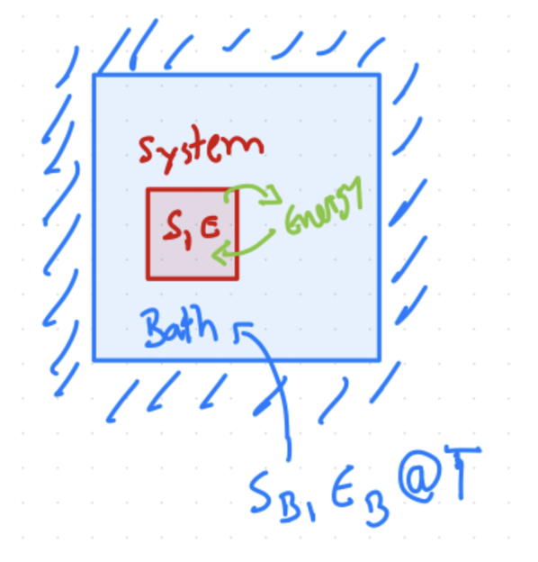
Fig. 3.1 Sketch of an NVT ensenble, held at a constant temperature $T$ by energy exchange with a bath.#

Consider system + bath:
- $S_{\text{total}} = S + S_B $
- $E_{\text{total}} = E + E_B $

Energy is exchanged so the system and bath come to $T$, as sketched in Fig. 3.1.

\[\begin{align*} S_B&=\frac{E_B+P_B V_B-\mu_B N_B}{T}=\frac{E_T-E+P_B V_B-\mu_B N_B}{T}=-\frac{E}{T}+\text { constants } \\ & S_T&=S-\frac{E}{T}+\text { constants } \end{align*}\]

The second law, $\text{max } S_T$, leads to

\[\begin{align*} \max_E \left[ S(E,V,N) - \frac{E}{T}\right] = \max_E \left[ - \frac{E-TS}{T}\right] = \max_E \left[ - \frac{A}{T}\right]\\ \rightarrow \min_E A \end{align*}\]

where $A(T,V,N)=E-TS$ is the Helmholtz free energy. Maximize $S_{\text{total}} \rightarrow $ minimize Helmholtz free energy!

The resulting fundamental equations are

\[\begin{align*} A = E - TS = -PV = \mu N \quad \text{with} \quad dA = -S\,dT - P\,dV + \mu\,dN \quad . \end{align*}\]

The same approach can be applied to exchange volume or number of particles with a bath. This then generates other thermodynamics potentials, $H(S,P,N)$, $G(T,P,N)$, etc. The internal energy ($U$), enthalpy ($H$), Helmholtz free energy ($A$), and Gibbs free energy ($G$) are all thermodynamic potentials.

3.1.1.1. Legendre Transforms and Thermodynamic Potentials#

A formal process to obtain these thermodynamic potentials is the Legendre Transform, a mathematical process to produce a new function wth a variable exchanged with its derivative. Used to exchange variables with their conjugate derivatives.

\[\begin{align*} \mathcal{L}_x\left[ f(x)\right] = g(p) = \max_x \left[ px = f(x)\right]= px^* -f (x^*) \end{align*}\]

where $x^*$ solves $f' (x^*)=p$.

In thermodynamics, we use a slightly different multivariable version:

\[\begin{align*} \mathcal{L}_x\left[ f(x,y,z)\right] = g(p,y,z) = \max_x \left[ f(x,y,z)-px\right]= f(x^*,y,z)- px^* \quad \end{align*}\]

where $x^*$ solves $\frac{\partial f (x^*,y,z)}{\partial x}=p$. Instead of $\max$ (for convcave), $\min$ can be also used (for convex).

For example, temperature (T) and entropy (S) are conjugate, as are pressure (P) and volume (V). The Legendre transform swaps these conjugate pairs.

Example: Helmholtz Free Energy

\[\begin{align*} S(E,V,N), \quad dS=\underbrace{\frac{1}{T}}_{"=p"} \underbrace{dE}_{"x"} + \frac{P}{T} dV - \frac{\mu}{T} dN \end{align*}\]

Now $\frac{1}{T} = \left(\frac{\partial S}{\partial E}\right)_{V,N}$.

\[\begin{align*} \mathcal{L}_E \left[ S(E,V,N) \right] = \max_E \left[ S(E,V,N) - \frac{E}{T}\right] = S(E^*) - \frac{E^*}{T} = \frac{A}{T} \end{align*}\]

Why this definition of $A$? Minimum $E$:

\[\begin{align*} E(S,V,N) \quad dE= TdS - PdV + \mu dN A(T,V,N) = \mathcal{L}_E \left[ E(S,V,N) \right] = min_S \left[ E(S,V,N) - TS \right] = E(S^*,V,N) - TS^* \quad. \end{align*}\]

In practice? Take conjugate variales, swap them, and add minus sign!

\[\begin{align*} d E &= TdS - PdV + \mu dN &\rightarrow dH &= TdS + VdP + \mu dN \\ d E &= TdS - PdV + \mu dN &\rightarrow dA &= -SdT -PdV +\mu dN \\ \end{align*}\]

folloing the same scheme:

\[\begin{align*} d H &= TdS + VdP + \mu dN &\rightarrow dG &= -SdT + VdP + \mu dN \\ d A &= -SdT -PdV +\mu dN &\rightarrow dG &= -SdT +VdP +\mu dN \\ \end{align*}\]

So $H=E+PV$ and $G=H-TS$.

Natural variables describe constraints; derivatives respond to satisfy the second law. The themodynamic potential is minimized when its natural variables are the constraint.

3.1.2. Microstates and Statistical Ensembles#

For simulations it is essential to understand the connections between macro- and microstates.

Macrostate: Defined by $E, V, N $, three variables.
Microstate: Specific configuration $(\vec{r}_N, \vec{p}_N)$, i.e all classical position and momenta. This means 6N coordinates!

there are many microstates correspond to the same macrostate. Not all microstates satisfy macroscopic constraints, e.g. not all $E(\vec{r}^N,\vec{p}^N)$ match the specified $E$.

The microstates evolve according to some physics, e.g. Newton’s equations.

\[\begin{align*} \dot{\vec{r}}_i = \frac{\vec{p}_i}{m_i}\\ \dot{\vec{p}}_i = -\frac{\partial U}{\partial r_i}\\ \end{align*}\]

An ensemble is the collection of all microstates consistent with the given constraints.

3.1.3. Time and Ensemble Averages#

Time average:
Sample one system over time, average: $\bar{f} = \frac{1}{N} \sum_{i=1}^N f(t_i)$.
Ensemble average:
Sample many systems at once, pull representative states $\langle f \rangle = \sum_v P_v f_v$, where $v$ are microstates, and $P_v$ is the probability of that state, and $f_v$ is the value of $f$ in that microstate.
If system is ergodic, time and ensemble averages are equivalent, that is, at long times it evolves through all microstates consistend with constraints, see Fig. 3.2.

Postulate of Equal A Priori Probabilities

In an isolated system (constant $E, V, N $), all accessible microstates are equally likely.

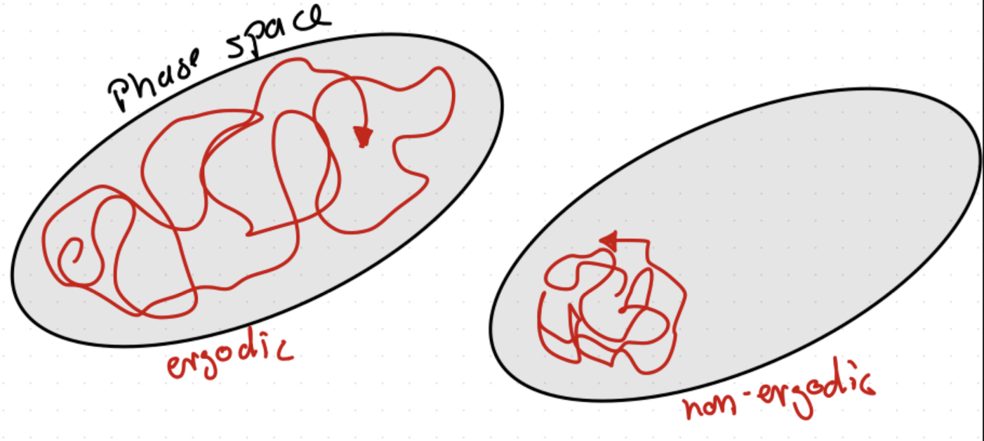
Fig. 3.2 Illustration of ergodic vs. non-ergodic.#

3.1.4. Microcanonical Ensemble (NVE)#

All microstates with energy $E $ are equally likely (as per postulate above).

Number of all microstates:
$\Omega(E, V, N) = \sum_v \delta(E - E_i)$ where $v$ are microstates.
Probability of a microstate:
$P_i = \frac{\delta(E - E_i)}{\Omega(E, V, N)}$. We call $\Omega$ the partition function for the ensembe, or the density of states.

From here, Boltzmann connected the macroscopic entropy to the microcanonical partition function:

Entropy:

\[\begin{align*} \boxed{ S = k_B \ln \Omega} \end{align*}\]

All thermodynamic properties can be derived from $\Omega$! $

\[\begin{align*} d \ln \Omega &= d(S/k_B) = \beta dE + \beta P dV - \beta \mu dN \\ \rightarrow \beta &= \left(\frac{\partial \ln \Omega}{\partial E}\right)_{V,N}\\ \rightarrow \beta P &= \left(\frac{\partial \ln \Omega}{\partial V}\right)_{E,N}\\ \rightarrow \beta \mu &= \left(\frac{\partial \ln \Omega}{\partial N}\right)_{E,V}\\ \end{align*}\]

$

3.1.5. Canonical Ensemble (NVT)#

Constant $E$ is inconvinient when comparing to experiments. What about constant $T$? This is a very common ensemble to operate in for both MD and MC simulations.

System exchanges energy with a heat bath at temperature $T$

Probability of a microstate:
$ P_i = \frac{e^{-\beta E_i}}{Z}$
Partition function:
$Z(T, V, N) = \sum_i e^{-\beta E_i}$
Average energy: $\langle E \rangle = -\frac{\partial \ln Z}{\partial \beta}$
Helmholtz free energy: $$ A = -k_B T \ln Z $$
In the thermodynamic limit: $$ \ln Z = -\beta A $$
Gibbs Entropy Formula: $$ S = -k_B \sum_i P_i \ln P_i $$
Substituting Boltzmann distribution: $$ S = k_B \ln Z + \beta \langle E \rangle = \frac{\langle E \rangle - A}{T} $$

3.1.6. Other Ensembles#

3.1.6.1. Isothermal-Isobaric (NPT)#

System exchanges energy and volume with a bath.
Probability: $$ P_i \propto e^{-\beta (E_i + P V_i)} $$
Partition function: $$ \Delta(T, P, N) = \sum_i e^{-\beta (E_i + P V_i)} $$
Gibbs free energy: $$ G = -k_B T \ln \Delta $$

3.1.6.2. Grand Canonical Ensemble (μVT)#

System exchanges energy and particles with a bath.
Probability: $$ P_i \propto e^{-\beta (E_i - \mu N_i)} $$
Partition function: $$ \Xi(T, V, \mu) = \sum_{N} \sum_i e^{-\beta (E_i - \mu N)} $$
Grand potential: $$ \Phi = -k_B T \ln \Xi $$

3.1.7. Additional Resources#

The Wikipedia pages for various thermodynamics and statistical mechanics topics are quite good:
- Wikipedia links for all Statmech Categories
- Wikipedia links for all Thermo Categories
Any statmech & thermo textboox